A PROBABILISTIC PRICE FORECASTING GUIDE WITH TECHNICAL ANALYSIS

Hidden Markov Model- A Statespace Probabilistic Forecasting Approach in Quantitative Finance

Application of Gaussian Mixture Model for Regime detection using historical NASDAQ Index time-series data

https://sarit-maitra.medium.com/membership

Hidden Markov Models (HMM) are proven for their ability to predict and analyze time-based phenomena and this makes them quite useful in financial market prediction. HMM can be considered mix of Brownian movements consisting of hidden layers and observed layers and comprising of sequence of events. In quantitative finance, the states of a system can be modeled as a Markov chain in which each state depends on the previous state in a non-deterministic way. In HMM these states are invisible, while observations which are the inputs of the model and depend on the visible states. HMM is typically used to predict the hidden regimes of observation data. The mathematical foundations of HMM were developed by Baum and Petrie in 1966.

The big question here is that, can we use the performances of stocks in the past to predict their future performances? The data with index seems to have similar behaviors on the same regimes. Thus, it is a natural instinct to analyze the stock behavioral pattern on a similar environment in the past to forecast its future outcomes. Based on this motivation, we will discuss how HMM can be used effectively to predict stock movements

Markov process is a process for which we can make predictions for the future based solely on its present state just as well as we could knowing the process’s full history [1].

Stock Price Prediction

We have seen the experimentation of a number of machine learning algorithms on stock prediction with varying degrees of success. We are also aware of the fact that, the price of the stock depends upon a multitude of factors and these factors mostly are hidden variables. The asset returns are comprised of multiple distributions. Time varying means and volatility normally comes from different distributions, regimes or states . Each regime has its own parameters e.g. regime can be stable with low volatility or regime could be risky with high volatility.

We have discussed earlier, how Statespace model & Kalman filter can be applied to predict stock movement. Here, in this article, we will see how Gaussian Mixture Model (GMM) can be used for regime selection. The selection will involve both the covariance type and the number of components in the model.

Historical NASDAQ data has been collected since 1970. When we call through API, the entire historical data from 1970 with 12341 rows and 5 columns. We will collect data from 1999 for our experiment. If you have better computing power, may use the entire data-set.

df = web.DataReader('^IXIC', data_source = 'yahoo', start = '2000-01-01')
print(df.head())
df.reset_index(inplace = True) #resetting index
print(df.head()) # display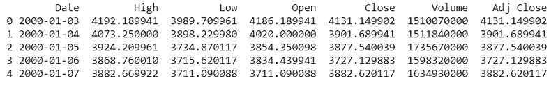

data = df[['High','Low','Open','Adj Close']]
data['pct_ret'] = data['Adj Close'].pct_change()
data.tail()
data['state'] = data['pct_ret'].apply(lambda x: 'up' if (x > 0.001)\
else ('down' if (x < -0.001)\
else 'no_change'))
data.tail()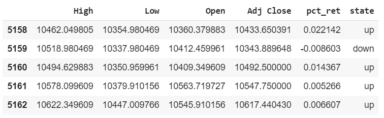

data['prev_state'] = data['state'].shift(1)
data.tail()

state_space = data[['prev_state', 'state']]
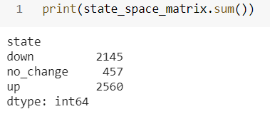
state_space_matrix = data.groupby(['prev_state', 'state']).size().unstack()
state_space_matrix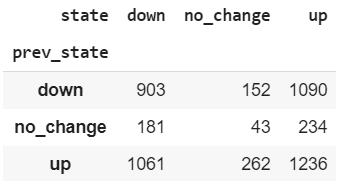

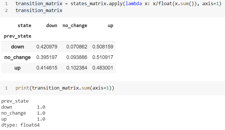
Let us create a function that maps transition probability data frame to Markov edges and weights

def _get_markov_edges(Q):
edges = {}
for col in Q.columns:
for idx in Q.index:
edges[(idx,col)] = Q.loc[idx,col]
return edges
edges_wts = _get_markov_edges(transition_matrix)
pprint(edges_wts)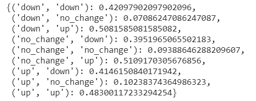

Graph object

states = ['up', 'down', 'no_change']
G = nx.MultiDiGraph()
# nodes correspond to states
G.add_nodes_from(state_space_matrix)
print(f'Nodes:\n{G.nodes()}\n')
# edges represent transition probabilities
for k, v in edges_wts.items():
tmp_origin, tmp_destination = k[0], k[1]
G.add_edge(tmp_origin, tmp_destination, weight=v, label=v)
print(f'Edges:')
pprint(G.edges(data=True))
pos = nx.drawing.nx_pydot.graphviz_layout(G, prog='dot')
nx.draw_networkx(G, pos)
edge_labels = {(n1,n2):d['label'] for n1,n2,d in G.edges(data=True)}
nx.draw_networkx_edge_labels(G , pos, edge_labels=edge_labels)
nx.drawing.nx_pydot.write_dot(G, 'nasdaq_markov.dot')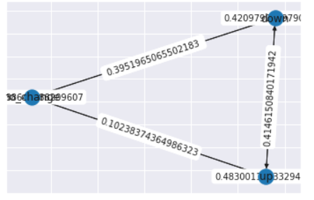

Feature engineering

In the current state, we have few features available for each day in the original data-set. These are the popular opening price, closing price, highest price, lowest price and volume. So, we will use them to compute the future price. In order to get more sequences and, more importantly, get a better understanding of the market’s behavior, we need to break-up the data into samples of sequences leading to different price patterns.

Therefore, instead of directly using the opening, closing, low, and high prices of a stock, we are going to extract some features using O,C,L,H,V and use them as predictor which will have all the logic to predict the price during a given day. to train our HMM. We can add more relevant features to add a robust model. Here, we will use below features to experiment and show how HMM works.

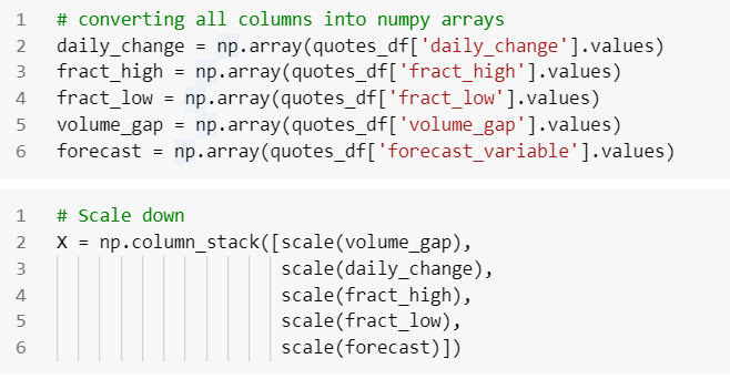
• volume gap = %change of volume
• daily change = (C-O)/O
• fractional high = (H-O)/O
• fractional low = (O-L)/O

We will create a simple model with reasonable predictive power. However, this is not for commercial use purpose.

Here, each predictor above will be treated as a sequence and will be used to train our model. So, we will have 4 chain of events as stated above on a particular day and we will use them to predict future ‘open’ price. Our goal here is to predict (t+1) value based on n (previous) days information. Therefore, defining the output value as forecast, which is a binary variable storing up or down values. We will predict ‘open’ price is up or down next day using the randomly sequence of events.

Let us write a function to create 100,00 randomly sequences looking at 10–30 trading days as event. Hence, we have taken 10–30 days as look-back period, which also can be modified to 50–60 days or so. So, it will be a binary classification problem and we will use each of events to train our HMM. The parameters are defined in below program.

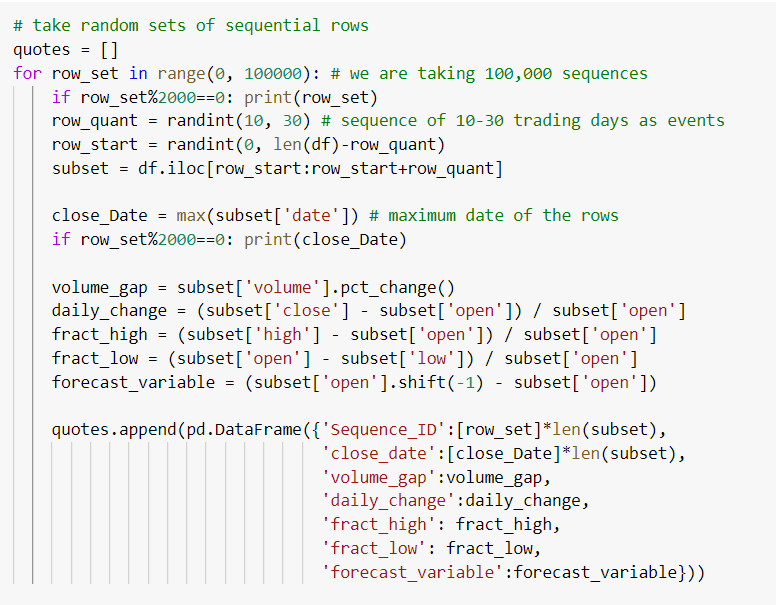
The above concept was taken from Manuel Amunategui who has provided an excellent idea of binning the data and doing binary classification by creating two transition matrices — a positive one and a negative one.

It takes some time to run considering 100,000 sequences and amount of data points we feed into the system. Here, our network architecture will look through the available data 100,000 times and sequence of 10–30 events to predict ‘open’ price up or down next day. We also have created our forecast variable which will see today’s price to predict tomorrow’s price.

In simpler Markov Chain, the state is directly visible to the observer, and therefore the state transition probabilities are the only parameters, while in the HMM, the state is not directly visible, but the output, dependent on the state, is visible. Each state has a probability distribution over the possible output. Therefore, the sequence generated by an HMM gives some information about the sequence of states…wikipedia

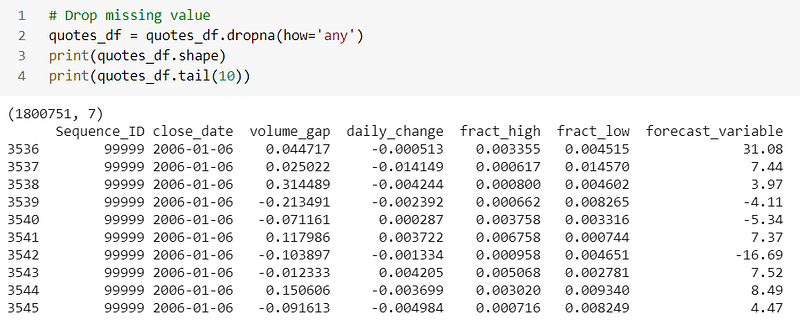
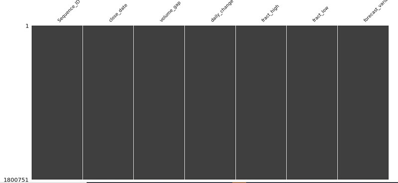
So, we collect all details in a data-frame as shown below. We concatenate all newly created columns in a data-frame and remove the null values.

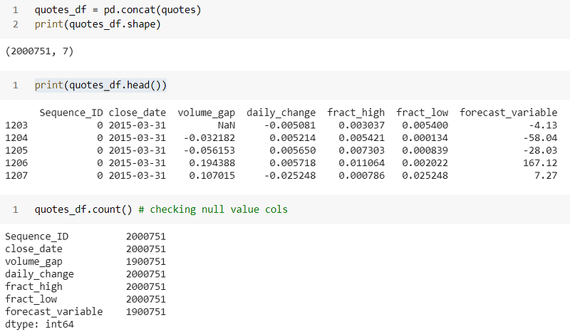
We drop here all the null values and print msno matrix to visualize that, our data-frame has no null values.

So, after having observations, we can compute using Bayesian network because out network knows now all the transition probabilities from one state to another. This is kind of similar to neural network here. Our HMM can know below three important things through our observations:

1. we can compute likelihood state from a sequence of observations.
2. we can work out the most probable sequence of states given the observations,
3. generate better HMM for our data given several state of observations.

Now, our first approach is to, using HMM to find regimes for the new variables. We use historical data of each variable to calibrate HMM parameters and to find the corresponding regimes. Let us convert the columns to numpy array and scale down the data.

Hidden Markov Model for regime detection

We will use historical data of each variable to calibrate HMM parameters and to find the corresponding regimes. The components are regimes here. Let us find out the optimum number of components using some information criteria. We will initiate a Gaussian Mixture model (GMM) to fit our time-series data with a range of 1–15 BIC to find the optimal number for our model. GMM employs an Expectation-Maximization (EM) algorithm to estimate regime and the likelihood sequence of regimes.

Gaussian mixture model is a probabilistic model that assumes all the data points are generated from a mixture of a finite number of Gaussian distributions with unknown parameters- ‘scikit-learn’

Optimal Number of Components using AIC/BIC

Choosing a number of hidden states for the HMM is a critical task. We will use standard criteria: the AIC and the BIC to examine the performances of HMM with different numbers of states. The two measures are suitable for HMM because, in the model training algorithm, the Baum–Welch algorithm, the EM method was used to maximize the log-likelihood of the model. We will limit numbers of states from two to four to keep the model simple and feasible for stock prediction. The AIC and BIC are calculated using the following formulas, respectively:

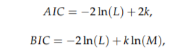
where L is the likelihood function for the model, M is the number of observation points, and k is the number of estimated parameters in the model. In this paper, we assume that the distribution corresponding to each hidden state is a Gaussian distribution. Therefore, the number of parameters, k, is formulated as k = N2 + 2N − 1, where N is numbers of states used in the HMM.

AIC and BIC

Both methods allow us to compare the relative suitability of different models. When choosing among a set of models we want to choose the AIC or BIC with the smallest information criterion value.

AIC rewards goodness of fit, but it also includes a penalty that is an increasing function of the number of estimated parameters. The penalty discourages over-fitting, because increasing the number of parameters in the model almost always improves the goodness of the fit — wikipedia

Both metrics implement a penalty; compared to AIC, BIC penalizes additional parameters more heavily and results in selecting fewer parameters. Gaussian Mixture comes with different options to constrain the covariance of the difference classes estimated e.g. spherical, diagonal, tied or full covariance. Here, we will do a grid search taking a range of components and try all the classes on the fitted GMM to identify number of optimal number of components based BIC score.

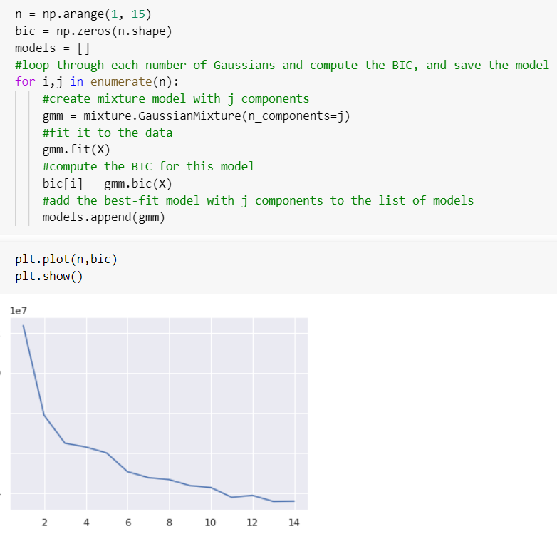
Here x-axis is number of Gaussian, y-axis is BIC; we can see that the BIC is minimized for 3 Gaussian, so the best model according to this method also has 3 components.We can see that, above function has identified 6 regimes.

Time series exhibit temporary periods where the expected means and variances are stable through time. These periods or regimes can be likened to hidden states.

Gaussian Mixture Model

Now, using the optimum number of 3 regimes, we will use the GMM to fit a model that estimates these regimes. We will initiate and fit a GMM to predict the hidden states using mean and variances. Depends on your computing speed, this might take some time to run.

The algorithm keeps track of the state with the highest probability at each stage. At the end of the sequence, the it will iterate backwards selecting the state that “won” each time step, and thus creating the most likely sequence of hidden states that led to the sequence of observations.

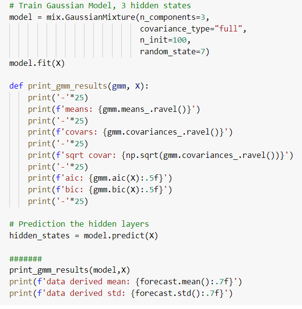
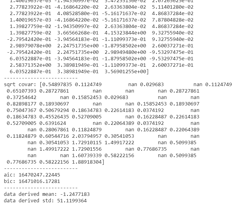
We see here that out model is based on Dynamic Bayesian Networks. The AIC & BIC values are quite close here. Finally, we will summarize the mean and variance of each observed variable on the corresponding regime. The performance of the indicators on each regime (in terms of center and spread) is given below.

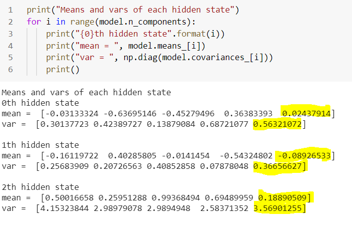
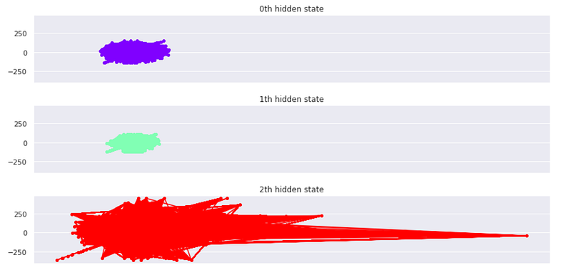
We see here that, each regime is characterized by means and covariances of the hidden states (regimes). Covarinaces part is the volatility indicator. The highlighted ones are the mean and variance of foretasted ‘open’ price. Let us go through each state to analyse the output.

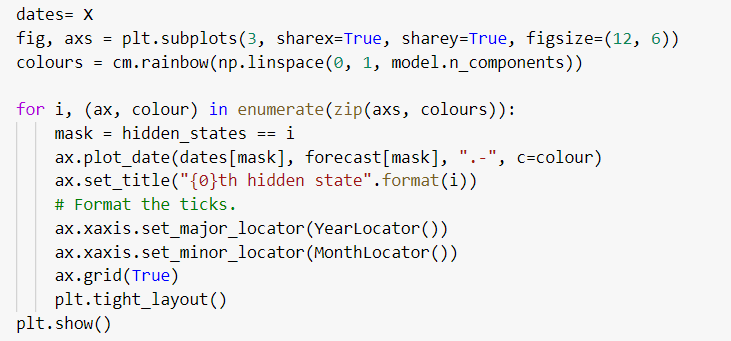
• 2th state is our largest opening price (0.188) but with highest variance (3.569) in the group which makes it high volatile regime. We can figure that out looking at the below plot as as well.
• 1th state opened with negative price (-0.089) and comparatively low variance (0.366).
• 0th state is with positive return (0.024) and lowest variance (0.563) in the group.

We can also assume that opening price will transition between these regimes based on probability. Our goal is to minimize the variance of return and then maximize the mean price.

An interesting visualization of Markov chain process that hop from one state to another, can be found here. Although, the mean-variance portfolio provides a foundation of modern finance theory and has numerous extensions and applications; however, it attracts maximum returns under a given risk. Optimal asset allocation across many assets is important and difficult.

Moreover, from the observations we can see that, that the stock market performs significantly different across different regimes. The momentum of a stock depends on many factors which includes corporate financial condition, management, overall economic condition and industry conditions, besides volatility other macroeconomic variables such as inflation (consumer price index), industrial production index etc. These factors and corresponding stock returns vary widely over different regimes. Moreover, long-term investments depend on the trends of these economic factors.

Summary

Bayesian network model is a statistical model and not a structural model and through this network, we general approach is to look back in time and measure relationship from there without taking into account what could potentially happen. However, the biggest advantage is that, we could encode assumptions through Bayesian network and statistical measures to take care of rarest of rare event could happen and possible could have an impact on forecasting.

Setting up optimization parameters and constraints to maximize the model performance is an important aspect of any forecasting model. I will discuss about optimization algorithm in a separate article.

I can be reached here.

Notice: The programs described here are experimental and should be used with caution. All such use at your own risk.

References:

1. Stochastic differential equations. In Stochastic differential equations, Øksendal, B. (2003), Springer, Berlin, Heidelberg. (pp. 65–84).
2. Scikit-learn: Machine Learning in Python, Pedregosa et al., JMLR 12, pp. 2825–2830, 2011
3. http://www.blackarbs.com/blog/introduction-hidden-markov-models-python-networkx-sklearn/2/9/2017
4. Nguyen, N., & Nguyen, D. (2015). Hidden Markov model for stock selection. Risks, 3(4), 455–473.
5. Nguyen, N. (2017). An analysis and implementation of the hidden Markov model to technology stock prediction. Risks, 5(4), 62.