
Hidden Markov Chain in brevity (Part 1 )
In this series, I will try my best to explain the probabilistic theory and computation behind Hidden Markov Chains (HMM) and how to fit problems into this stochastic model. I hope that you will have a clearer understanding on how this powerful statistical model works, and thus be able to think of more real life applications of HMM.
I have broken this series down to 3 parts, which represent the 3 fundamental processes for building a HMM. (Rabiner, 1989)
- Intro + Likelihood evaluation problem,
- Decoding problem
- Learning problem
For now, I seek your understanding to hold on to these problems, their explanation and relevance will soon be clear in the respective sections.
Introduction to Markov Chains
The HMM is one of the most important machine learning models in speech and language processing. To define it properly, we need to first introduce the Markov chain, sometimes called the observed Markov model.
So what are Markov Chains (MM) and how are they relavant? The MM is a sequence model. A sequence model is a model whose job is to assign a label or class to each unit in a sequence, thus mapping a sequence of observations to a sequence of labels. A MM is a probabilistic sequence model: given a sequence of units (words, letters, morphemes, sentences), they compute a probability distribution over possible sequences of labels and choose the best label sequence.
A common example of MM in our daily lives is the predictive text feature in messaging apps. This feature is common in any messaging platform and I am sure you have wondered how it works, and how it is able to learn from your texting patterns to suggest words to you.

Sentences are a form of sequential data, and this is where MM excels. What comes after a particular word with the highest probability is a problem that Markov chains can solve.
In the diagram below, we can see that a Markov chain is a kind of probabilistic graphical model: a way of representing probabilistic assumptions in a graph. On the left, it models the transition states {Hot, Warm, Cold} of weather, and the right is the autocomplete example where it models the transition states of words {Is, Snow, White}.
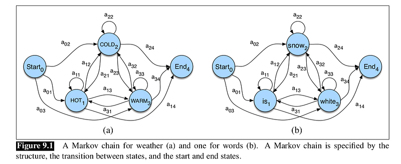
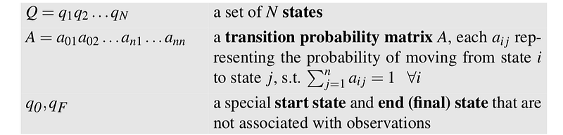
A Markov chain is specified by the following components:
You can check out a very easily understandable visualization I found: http://setosa.io/ev/markov-chains/
The Hidden Markov Model
A Markov chain is useful when we need to compute a probability for a sequence of events that we can observe in the world. In many cases, however, the events we are interested in may not be directly observable in the world. For example, in the weather data set, we may not have the direct data of weather {Hot, Warm, Cold}, they are hidden from us. However, let’s say we have a surrogate (related) observed variable, such as the number of ice-cream that were sold on each time period. We can build a statistical model to infer the weather (hidden data) from the number of ice-cream sold (observed data). Thus this is where HMM excels in, modeling the unseen from the seen.
Let’s begin with a formal definition of a hidden Markov model, focusing on how it differs from a Markov chain. An HMM is specified by the following components:
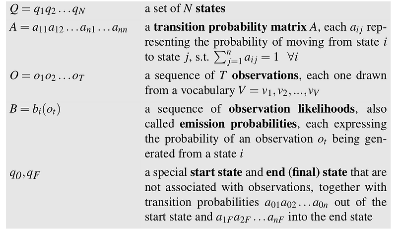
The difference here between MM and HMM is the addition of a observable layer, while our states are suppressed underneath it to be hidden. The observed variables and their respective observation likelihood are O and B as shown above.
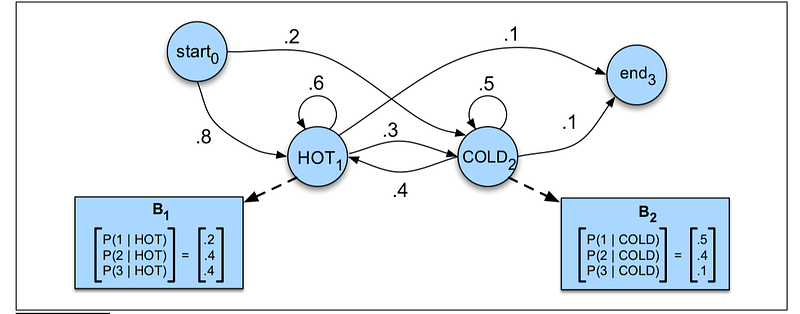
The diagram below shows a sample HMM for the ice cream task. The two hidden states (H and C) correspond to hot and cold weather, and the observations (drawn from the alphabet O = {1, 2, 3}) correspond to the number of ice creams sold on a given day.
Problem 1: Likelihood Evalution
So herein is the first problem that we would like to solve using a HMM, the likelihood evaluation problem. It is formally defined as: Given an HMM λ = (A, B) and an observation sequence O, determine the likelihood P(O|λ ).
For a Markov chain, where the surface observations are the same as the hidden events, we could compute the probability of 3 1 3 just by following the states labeled 3 1 3 and multiplying the probabilities along the arcs. For a hidden Markov model, things are not so simple. We want to determine the probability of an ice-cream observation sequence like 3 1 3, but we don’t know what the hidden state sequence is!
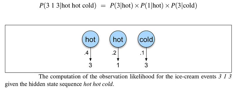
Let’s start with a slightly simpler situation. Suppose we already knew the weather and wanted to predict how much ice cream will be sold. This is a useful part of many HMM tasks. For a given hidden state sequence (e.g., hot hot cold), we can easily compute the output likelihood of 3 1 3. First, recall that for hidden Markov models, each hidden state produces only a single observation. Thus, the sequence of hidden states and the sequence of observations have the same length. Given this one-to-one mapping and the Markov assumptions expressed, for a particular hidden state sequence Q = q0,q1,q2,...,qT and an observation sequence O = o1 , o2 , ..., oT , the likelihood of the observation sequence is the total conditional probability of the observations given the hidden state summed up over the whole time period. P(O|Q) = Total product of P(o_i|q_i)
The computation of the forward probability for our ice-cream observation 3 1 3 from one possible hidden state sequence hot hot cold is shown. Below is a graphic representation of this computation.
But of course, we don’t actually know what the hidden state (weather) sequence was. We’ll need to compute the probability of ice-cream events 3 1 3 instead by summing over all possible weather sequences, weighted by their probability. First, let’s compute the joint probability of being in a particular weather sequence Q and generating a particular sequence O of ice-cream events. In general, this is
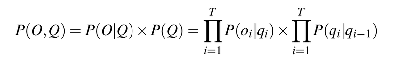
The computation of the joint probability of our ice-cream observation 3 1 3 and one possible hidden state sequence hot hot cold is P(313,hot hot cold) = P(hot|start)×P(hot|hot)×P(cold|hot) ×P(3|hot) × P(1|hot) × P(3|cold). Now that we know how to compute the joint probability of the observations with a particular hidden state sequence, we can compute the total probability of the observations just by summing over all possible hidden state sequences:
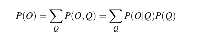
For our particular case, we would sum over the eight 3-event sequences cold cold cold, cold cold hot, cold hot cold, … For an HMM with N hidden states and an observation sequence of T observa- tions, there are N^T possible hidden sequences. For real tasks, where N and T are both large, N^T is a very large number, so we cannot compute the total observation likelihood by computing a separate observation likelihood for each hidden state sequence and then summing them. Instead of using such an extremely exponential algorithm, we use an efficient O(N^2 * T ) algorithm called the forward algorithm
Forward Algorithm
The forward algorithm is a dynamic programming algorithm, where we use past computed values to calculate the next stage in the observable sequence. It computes the observation probability by summing over the probabilities of all possible hidden state paths that could generate the observation sequence, but it does so efficiently by implicitly compressing each of these paths into a single forward trellis.
The figure below shows an example of the forward trellis for computing the likelihood of 3 1 3 given the hidden state sequence hot hot cold.
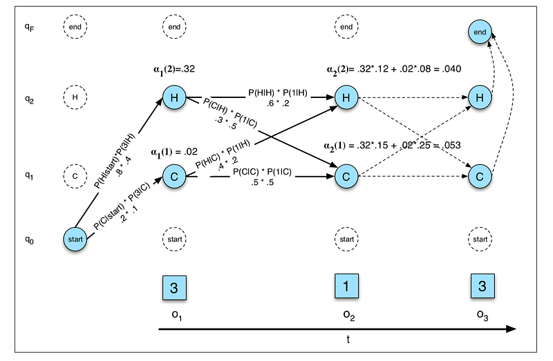
Each cell of the forward algorithm trellis αt ( j) represents the probability of being in state j after seeing the first t observations, given the emission probabilities λ . The value of each cell αt ( j) is computed by summing over the probabilities of every path that could lead us to this cell. Formally, each cell expresses the following probability:
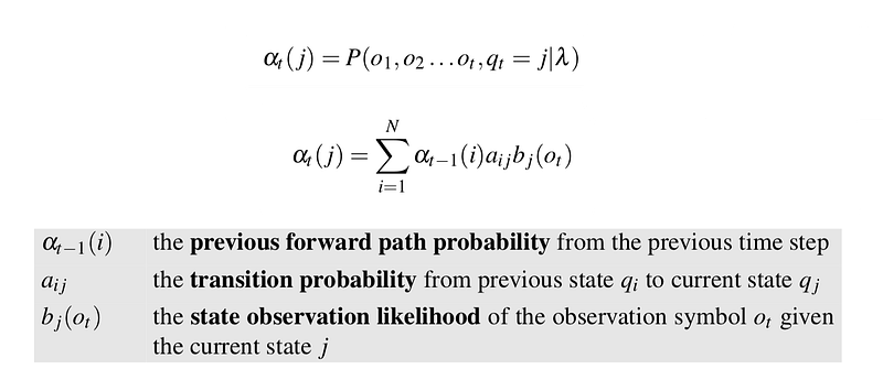
From this, we can compute efficiently the likelihood of a sequence of observed events, by calculating the probability from the start and propagate it forward through the sequence, and having all the past information be compressed in a current trellis, before moving on to the next and calculating as we move along linear time. The recursive iteration algorithm can be structured in the following way:
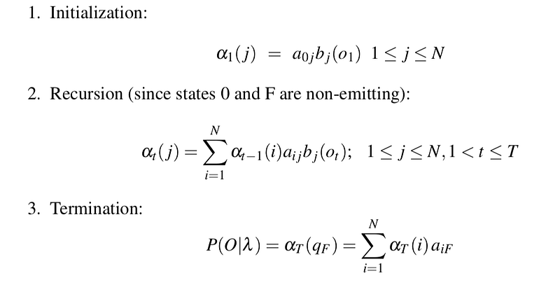
Hence, we can finally compute P(O|lambda) in an efficient manner, and thus solve the first problem of HMM. For the next 2 sections, it will focusing on the decoding and learning problems which are: what hidden sequence will best fit an observed sequence, and how do we find the parameters of the model in an unsupervised way.
Thanks for coming to the end of this article. I know, this was definitely not in brevity at all, and I apologise. It is almost impossible to compress all the fundamental math details without compromising on the logical flow. Maybe for the next few parts will need to exclude that word from my title (:
Till next time folks
References: Speech and Language Processing. Daniel Jurafsky & James H. Martin, Stanford