
Harnessing Fama-French Models for Enhanced Algorithmic Trading Strategies
A Comprehensive Guide to Integrating Statistical Models with Python for Predictive Trading.
In the realm of algorithmic trading, the fusion of statistical modeling and advanced programming opens new avenues for market analysis and strategy development. This article delves into the practical application of the renowned Fama-French 3-Factor and 5-Factor Models within a Python-based trading framework. We begin by setting up our Python environment with essential libraries such as Pandas, NumPy, and Matplotlib, which facilitate data manipulation, statistical analysis, and visualization, respectively. The core of our exploration revolves around processing financial datasets, utilizing linear regression techniques, and generating predictive trading signals based on these robust economic models. By seamlessly integrating these models into our algorithmic trading strategy, we aim to uncover deeper insights into stock returns and market behavior, thereby enhancing our portfolio’s predictive accuracy and performance. Through this technical guide, readers will gain hands-on experience in applying these sophisticated models in a structured and efficient manner, paving the way for more informed and data-driven trading decisions.
Let’s start coding:
# Initial Imports:
import pandas as pd
import numpy as np
from pathlib import Path
from datetime import datetime
import warnings
warnings.filterwarnings('ignore')

# To run models:
import statsmodels.api as sm
from sklearn.ensemble import RandomForestClassifier
from sklearn.datasets import make_classification
from joblib import dump, load

# For visualizations:
import matplotlib.pyplot as plt
import seaborn as sns
%pylab inline
%matplotlib inline
The code is an initialization script for a Python-based algorithmic trading project, which is set up to test and examine the Fama-French 3-Factor and 5-Factor Models. These models are used in financial economics to describe stock returns. The initial imports bring in several Python libraries necessary for the projects operations. Pandas and NumPy are used for data manipulation and numerical operations. Path from pathlib and datetime are for handling file paths and dates, respectively.
The warnings library is used to suppress warnings that might clutter the output. For running the economic models and machine learning algorithms, the code imports the statsmodels library for statistical modeling, the RandomForestClassifier for classification tasks using a machine learning ensemble method, and functions for creating synthetic classification data and saving/loading models. Lastly, for data visualization, the code draws in matplotlib, a plotting library, and seaborn which is a statistical visualization library. It also contains IPython magic commands to enable inline plotting within a Jupyter notebook environment, ensuring that graphs and plots are displayed directly below the code cells that produce them.
The purpose of this code snippet is to set up the necessary environment for conducting algorithmic trading based on the Fama-French models by loading the appropriate Python libraries and configuring the environment. This would usually be the first step in a script or notebook designed to analyze the stock market and predict portfolio returns using established economic factors.
Pre-Processing
3-Factor Model
# Define function to read in factors from csv and return cleaned dataframe:
def get_factors(factors):
  factor_file=factors+".csv"
  factor_df = pd.read_csv(factor_file)

  # Clean factor dataframe:
  factor_df = factor_df.rename(columns={
    'Unnamed: 0': 'Date',
  })

  factor_df['Date'] = factor_df['Date'].apply(lambda x: pd.to_datetime(str(x), format='%Y%m%d'))

  # Set "Date" as Index:
  factor_df = factor_df.set_index('Date')

  return factor_df
The Python code defines a function named get_factors that takes a string input presumed to be a name of a factor and uses this string to locate a .csv file containing factor data related to the Fama-French models. The function then reads this CSV file into a pandas DataFrame and performs a series of data cleaning steps. The first step of the cleaning process is to rename a column that is presumably the date column but unnamed in the original file. The function changes this columns name to Date.
Next, it converts the values in the Date column to Python datetime objects, ensuring they are in the YYYYMMDD format, which is essential for time-series analysis. After the dates are properly formatted, the code sets the Date column as the index of the DataFrame, which is a common practice when working with time-series data to facilitate time-based indexing and analysis. Finally, the cleaned DataFrame is returned.
This function is helpful within the broader context of an Algorithmic Trading project that examines the Fama-French 3-Factor Model and the Fama-French 5-Factor Model as it prepares the necessary data to further analyze and predict portfolio returns.
# Confirm Fama-French dataframe:
factors = get_factors("french_fama")
factors.head()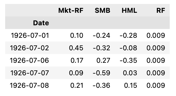
This Python code snippet is a part of an Algorithmic Trading project related to analyzing financial models, specifically the Fama-French 3-Factor and the 5-Factor models. These models are designed to help explain stock returns through various market factors.
The code performs two main functions:
- It retrieves a dataset containing Fama-French factors. This is done with the function get_factorsfrench_fama, where french_fama likely indicates the specific set of factors or the source of the data. This function could be one defined elsewhere in the code or part of a library for financial data analysis.
- It then previews the initial few rows of the dataset using factors.head. This is a common method used in data analysis to get a quick look at the structure and some sample data from the dataset for verification and initial understanding.
# Do same thing as above, but for the individual stock CSV:
def choose_stock(ticker):
  ticker_file=ticker+".csv"
  stock=pd.read_csv(ticker_file, index_col='Date', parse_dates=True, infer_datetime_format=True)
  stock["Returns"]=stock["Close"].dropna().pct_change()*100
  stock.index = pd.Series(stock.index).dt.date

  return stock
The code defines a Python function named choose_stock that takes a ticker symbol as its argument. The purpose of this function is to load historical stock data from a CSV file corresponding to the given ticker symbol, calculate the daily percentage returns of the stock, and return the processed stock data.
When invoked, the function constructs the filename of the CSV by appending .csv to the ticker symbol. It then reads this CSV file into a pandas DataFrame, ensuring that the Date column is used as the index and that the dates are properly parsed. After loading the data, it calculates the daily percentage change in the closing price of the stock, multiplies it by 100 to express it as a percentage, and adds these returns as a new column to the DataFrame.
Finally, the function converts the DataFrame index to a Python date object for easier handling and returns the modified DataFrame. This function is a utility within a larger algorithmic trading project that focuses on examining different Fama-French models to predict the returns of a portfolio. By isolating the process of loading and preparing an individual stocks data, the function aids in the analysis of single stocks against these models.
# Read in ATT dataframe using above function:
ticker="T"
stock=choose_stock(ticker)
stock.head()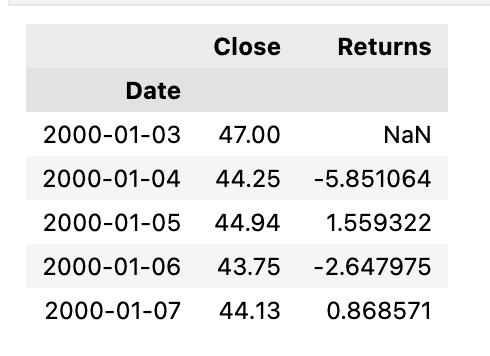
The Python code snippet is designed to retrieve and display the first few rows of a stock data frame, specifically for the stock with the ticker symbol T, which typically represents AT&T Inc. This is done as part of an Algorithmic Trading project which investigates the predictive power of the Fama-French 3-Factor and 5-Factor models on portfolio returns.
In this snippet, a function choose_stock is called with the argument ticker, set to the string T. This function is presumably defined elsewhere in the project and is responsible for obtaining the stock information from a data source. After calling the choose_stock function, an object named stock is created, containing the data frame with the AT&T stock information. By calling the head method on this stock data frame, the code displays the first five rows of the data frame.
These rows typically include essential information such as the date, opening price, closing price, volume, and possibly other custom analytical metrics relevant to the project. The purpose of this snippet is to briefly show a preview of the AT&T stock data and ensure that the data has been loaded correctly into the data frame for further analysis within the context of the Fama-French models evaluation. These models are used in financial economics to explain stock returns by considering market risk factors.
# Concatenate Fama-French dataframe with Stock dataframe:
combined_df = pd.concat([factors, stock], axis='columns', join='inner')

# Drop nulls:
combined_df = combined_df.dropna()
combined_df = combined_df.drop('RF', axis=1)

# Preview dataframe:
combined_df.head()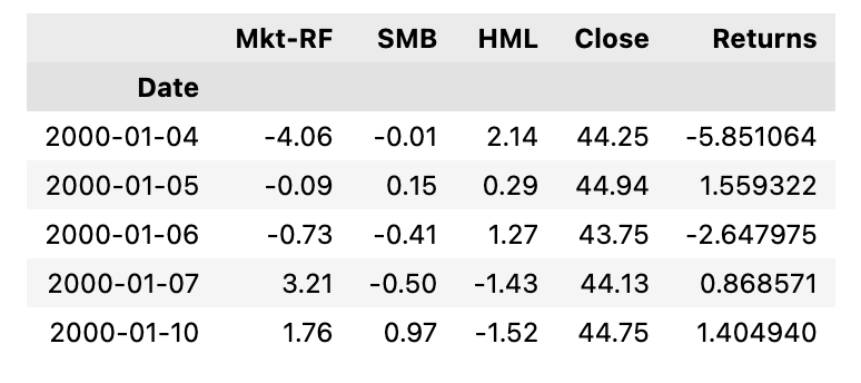
This Python code snippet is designed to merge two dataframes: one containing Fama-French factors and the other containing stock data. This is achieved through the use of the pandas librarys concat function, which combines the two dataframes column-wise and only includes rows that have matching index values in both dataframes an inner join. After the concatenation, the code ensures data cleanliness by removing any rows that contain missing values with the dropna method.
This step is critical in preparing the data for accurate and meaningful analysis in the context of algorithmic trading, particularly when assessing financial models like the Fama-French 3-Factor and 5-Factor Models. Then, the code removes the column labeled RF, which likely stands for the risk-free rate, a component typically accounted for in the Fama-French models but may not be needed for the specific analysis intended here.
Lastly, a preview of the resulting combined dataframe is requested by calling the head method, which by default displays the first five rows. This serves as a quick check to ensure that the previous operations have been executed correctly and the dataframe is ready for further analysis in the trading algorithm. The code is aimed at data preparation, a crucial step in the pipeline of algorithmic trading strategy development.
# Define X and y variables:
X = combined_df.drop('Returns', axis=1)
X = X.drop('Close',axis=1)
y = combined_df.loc[:, 'Returns']
This Python code is concerned with preparing the data that will likely be used for running regression analyses as part of examining the Fama-French 3-Factor and 5-Factor Models for predicting portfolio returns. The code performs data preprocessing by setting up the independent variables \X\ and the dependent variable \y\ using data from a presumably pre-existing DataFrame named combined_df.
The independent variables are being set up by removing the column labeled Returns and the column labeled Close from combined_df to create the \X\ variable. The Returns column is the dependent variable and represents the portfolio returns that the Fama-French models aim to predict. The column labeled Close probably contains the closing prices of stocks or assets and is not needed for the model inputs.
Subsequently, the dependent variable \y\ is created by selecting only the Returns column from combined_df. In summary, the purpose of this code is to structure the data into a format that is suitable for feeding into a statistical model or machine learning algorithm to investigate the relationship between the factors outlined by the Fama-French models and the portfolio returns.
# Split into Training/Testing Data:
split = int(0.8 * len(X))
X_train = X[: split]
X_test = X[split:]
y_train = y[: split]
y_test = y[split:]
close_test=combined_df["Close"][split:]
close_test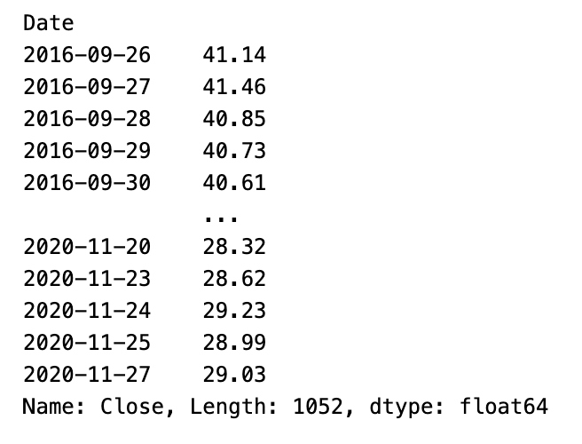
The provided Python code snippet is designed to split datasets into training and testing subsets for the purpose of validating the performance of the Fama-French 3-Factor and 5-Factor models in an algorithmic trading context. The models aim to explain and predict portfolio returns based on different financial factors.
The snippet first calculates the index at which to split the dataset, this index is determined as 80% of the length of the dataset denoted by X. It then uses this index to separate X the set of independent variables or features and y the dependent variable or target, which in this context would be the portfolio returns into training and test sets. Training sets X_train and y_train will be used to fit the models, while test sets X_test and y_test will be used to evaluate the models predictive performance.
Additionally, the code selects the Close prices from a dataframe combined_df, corresponding to the test set period, most likely for further analysis or comparison with the model predictions. This Close data could be used to compare the actual closing prices of assets with predicted values obtained from the model applied to X_test.
# Import Linear Regression Model from SKLearn:
from sklearn.linear_model import LinearRegression

# Create, train, and predict model:
lin_reg_model = LinearRegression(fit_intercept=True)
lin_reg_model = lin_reg_model.fit(X_train, y_train)
predictions = lin_reg_model.predict(X_test)
The provided code snippet is about implementing a linear regression model using scikit-learn, a machine learning library for Python. This is a common approach in financial analyses, specifically here in the context of the Fama-French factor models, which are used to describe stock returns. The code starts by importing the LinearRegression class from the scikit-learn library.
It then creates an instance of this class with fit_intercept=True, which means the model will calculate the intercept term in the regression equation. Next, it trains the model by passing training data X_train and y_train where X_train contains the independent variables that are believed to explain the portfolio returns and y_train has the dependent variable, or the actual portfolio returns.
After fitting the model to the training data, the code uses the trained model to predict values on a separate dataset X_test, which likely contains similar factors but from different time frames or assets, allowing the user to evaluate the models performance. These predictions can be compared with the actual returns to assess how well the Fama-French model explains or predicts stock returns in the context of algorithmic trading.
# Convert y_test to a dataframe:
y_test = y_test.to_frame()
The code snippet provided converts the y_test variable, which represents test data, into a pandas DataFrame. This is commonly done in data analysis and machine learning tasks in Python, where pandas DataFrames are a preferred structure for handling tabular data due to their flexibility and rich functionality. In the context of an Algorithmic Trading project, the y_test data likely contains actual portfolio returns that are used to test the models predictions.
The model, based on the Fama-French 3-Factor or the Fama-French 5-Factor Model, aims to explain stock returns through various economic factors. By converting y_test into a DataFrame, it can be more easily compared to the predicted returns generated by these models, likely facilitating further analysis such as calculating metrics to evaluate model performance.
signals_df = y_test.copy()

# Add "predictions" to dataframe:
y_test['Predictions'] = predictions
y_test["Close"]=close_test

# Add "Buy Signal" column based on whether day's predictions were greater than the day's actual returns:
y_test['Buy Signal'] = np.where(y_test['Predictions'] > y_test['Returns'], 1.0,0.0)

# Drop nulls:
y_test=y_test.dropna()

y_test.head()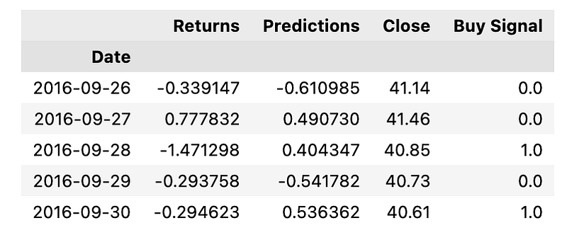
The provided Python code is used as part of an algorithmic trading project to handle finance data with the purpose of generating trading signals. It makes use of a testing dataset y_test that likely includes the actual returns of a portfolio.
The code does the following:
- Copies the y_test dataframe to another dataframe called signals_df, presumably for preserving the original test data.
- The variable predictions, which appears to contain predicted returns presumably from a Fama-French model, is added to the y_test dataframe.
- The actual close prices of the assets close_test are also added to the y_test dataframe.
- It then computes a Buy Signal by comparing the predicted returns with the actual returns. If the prediction is greater, it marks a 1.0 indicating a buy signal, otherwise a 0.0 indicating no buy signal.
- The dataframe is cleaned by dropping any rows containing null values.
- Finally, it displays the first few rows of the modified y_test dataframe, now including the additional columns for predictions and buy signals, by using .head for quick inspection.
The overall purpose of this code is to enrich the dataset with predictive information and trade signals to inform trading decisions within an algorithmic trading strategy.
# Define function to generate signals dataframe for algorithm:
def generate_signals(input_df, start_capital=100000, share_count=2000):
  # Set initial capital:
  initial_capital = float(start_capital)

  signals_df = input_df.copy()

  # Set the share size:
  share_size = share_count

  # Take a 500 share position where the Buy Signal is 1 (prior day's predictions greater than prior day's returns):
  signals_df['Position'] = share_size * signals_df['Buy Signal']

  # Make Entry / Exit Column:
  signals_df['Entry/Exit']=signals_df["Buy Signal"].diff()

  # Find the points in time where a 500 share position is bought or sold:
  signals_df['Entry/Exit Position'] = signals_df['Position'].diff()

  # Multiply share price by entry/exit positions and get the cumulative sum:
  signals_df['Portfolio Holdings'] = signals_df['Close'] * signals_df['Entry/Exit Position'].cumsum()

  # Subtract the initial capital by the portfolio holdings to get the amount of liquid cash in the portfolio:
  signals_df['Portfolio Cash'] = initial_capital - (signals_df['Close'] * signals_df['Entry/Exit Position']).cumsum()

  # Get the total portfolio value by adding the cash amount by the portfolio holdings (or investments):
  signals_df['Portfolio Total'] = signals_df['Portfolio Cash'] + signals_df['Portfolio Holdings']

  # Calculate the portfolio daily returns:
  signals_df['Portfolio Daily Returns'] = signals_df['Portfolio Total'].pct_change()

  # Calculate the cumulative returns:
  signals_df['Portfolio Cumulative Returns'] = (1 + signals_df['Portfolio Daily Returns']).cumprod() - 1

  signals_df = signals_df.dropna()

  return signals_df
The Python code provided is part of an algorithmic trading project that aims to facilitate the trading of financial securities based on the Fama-French 3-Factor and 5-Factor models. The purpose of the code is to create a dataframe that generates trading signals and tracks the performance of a trading portfolio over time.
The function generate_signals takes a dataframe input_df containing financial data alongside two optional parameters for setting the initial capital and the number of shares to be taken in a position. It starts by making a copy of the input dataframe to avoid modifying the original data and sets the initial capital and share size. Within this dataframe, based on a column named Buy Signal, the function calculates and records when to enter buy or exit sell a position, which is defined as purchasing or selling a fixed number e.g., 500 of shares.
The code computes various financial metrics such as the position in shares, cash in the portfolio, holdings value of owned shares, total value of the portfolio, and the portfolio’s daily and cumulative returns. By tracking these metrics, the code provides insights into the trading strategys effectiveness, which includes the evaluation of how the portfolios value changes over time in response to the computed buy or sell signals. This is crucial for assessing the performance of the trading strategy based on the historical data, and for potentially optimizing the strategy for future use in live trading scenarios.
# Generate and view signals dataframe using generate signals function
signals_df=generate_signals(y_test)
signals_df.head(10)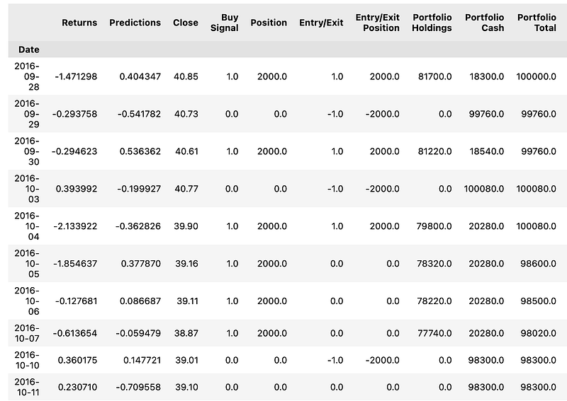
This Python code snippet is used for generating trading signals based on predictive models, particularly within the context of algorithmic trading influenced by the Fama-French 3-Factor and 5-Factor models. These models are widely used in finance to describe stock returns in relation to three or five different risk factors, respectively.
The code calls a function named generate_signals, which appears to take as input y_test. Though not shown, y_test might contain historical data, test data, or future returns as predicted by either the 3-Factor or 5-Factor model, or some variation thereof. The generate_signals function processes this input and returns a dataframe containing trading signals.
After generating the signals dataframe, the code proceeds to display the first 10 rows of this dataframe using the head method, which is a common function in the pandas library for previewing the top rows of a dataframe. The purpose of displaying these rows is likely to perform a quick visual check to ensure that the signal generation is functioning as expected before utilizing these signals in live trading decisions or further analysis.
def algo_evaluation(signals_df):
  # Prepare dataframe for metrics
  metrics = [
      'Annual Return',
      'Cumulative Returns',
      'Annual Volatility',
      'Sharpe Ratio',
      'Sortino Ratio']

  columns = ['Backtest']

  # Initialize the DataFrame with index set to evaluation metrics and column as `Backtest` (just like PyFolio)
  portfolio_evaluation_df = pd.DataFrame(index=metrics, columns=columns)
  # Calculate cumulative returns:
  portfolio_evaluation_df.loc['Cumulative Returns'] = signals_df['Portfolio Cumulative Returns'][-1]
  # Calculate annualized returns:
  portfolio_evaluation_df.loc['Annual Return'] = (signals_df['Portfolio Daily Returns'].mean() * 252)
  # Calculate annual volatility:
  portfolio_evaluation_df.loc['Annual Volatility'] = (signals_df['Portfolio Daily Returns'].std() * np.sqrt(252))
  # Calculate Sharpe Ratio:
  portfolio_evaluation_df.loc['Sharpe Ratio'] = (signals_df['Portfolio Daily Returns'].mean() * 252) / (signals_df['Portfolio Daily Returns'].std() * np.sqrt(252))

  #Calculate Sortino Ratio/Downside Return:
  sortino_ratio_df = signals_df[['Portfolio Daily Returns']].copy()
  sortino_ratio_df.loc[:,'Downside Returns'] = 0

  target = 0
  mask = sortino_ratio_df['Portfolio Daily Returns'] < target
  sortino_ratio_df.loc[mask, 'Downside Returns'] = sortino_ratio_df['Portfolio Daily Returns']**2
  down_stdev = np.sqrt(sortino_ratio_df['Downside Returns'].mean()) * np.sqrt(252)
  expected_return = sortino_ratio_df['Portfolio Daily Returns'].mean() * 252
  sortino_ratio = expected_return/down_stdev

  portfolio_evaluation_df.loc['Sortino Ratio'] = sortino_ratio


  return portfolio_evaluation_df
The code defines a function algo_evaluation that takes a DataFrame signals_df as input, which contains the daily returns of a trading portfolio. The purpose of this code is to evaluate the performance of an algorithmic trading strategy by calculating various performance metrics commonly used in the financial industry.
The code initializes a new DataFrame with performance metrics as index rows which include Annual Return, Cumulative Returns, Annual Volatility, Sharpe Ratio, and Sortino Ratio. These metrics are indicative of the portfolios overall performance and risk-adjusted returns. The function calculates the cumulative returns, annualized returns, and annual volatility of the portfolio by performing operations on the daily returns data contained within the input DataFrame.
Additionally, the code computes the Sharpe Ratio, which is used to understand the return of an investment compared to its risk. It is calculated as the average return earned in excess of the risk-free rate per unit of volatility or total risk. Lastly, the code assesses the Sortino Ratio, which is similar to the Sharpe Ratio but only considers downside volatility, which is more relevant for investors who are concerned about downside risks.
Finally, the function algo_evaluation returns a DataFrame that summarizes all these calculated performance metrics, thus providing a quick snapshot of the trading strategys performance based on historical data. This output can be used to compare different trading strategies or evaluate the effectiveness of a single strategy over time.
# Generate Metrics for Algorithm:
algo_evaluation(signals_df)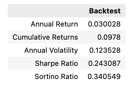
The Python function algo_evaluationsignals_df appears to be part of a larger code related to algorithmic trading, specifically focused on evaluating the performance of an algorithm that applies the Fama-French 3-Factor and 5-Factor Models. These models are used in financial economics to describe how stocks returns are affected by three or five different types of economic risk, respectively.
The function takes as input a data frame signals_df, which likely contains the signals or trading decisions generated by the investment algorithm based on those models. These signals could for instance mark when to buy or sell a particular asset, and they may also include associated data, such as expected returns, factor exposures, or other relevant metrics. The purpose of algo_evaluation is to assess these algorithm-generated signals and calculate various performance metrics.
These metrics might include the algorithms profitability, risk-adjusted returns, accuracy of predictions, and adherence to the Fama-French models premises.
Overall, the function is a tool for backtesting, which is a method for understanding how well a trading strategy would have done historically. By using this function, one can critically evaluate the algorithms effectiveness and make decisions about its utility for future trading.
# Define function to evaluate the underlying asset:
def underlying_evaluation(signals_df):
  underlying=pd.DataFrame()
  underlying["Close"]=signals_df["Close"]
  underlying["Portfolio Daily Returns"]=underlying["Close"].pct_change()
  underlying["Portfolio Daily Returns"].fillna(0,inplace=True)
  underlying['Portfolio Cumulative Returns']=(1 + underlying['Portfolio Daily Returns']).cumprod() - 1

  underlying_evaluation=algo_evaluation(underlying)

  return underlying_evaluation
This Python code defines a function named underlying_evaluation, which is used to analyze the performance of a financial asset based on its closing prices over a period of time. The code utilizes a data structure known as a pandas DataFrame to manipulate and analyze the data. The function takes a DataFrame signals_df as input.
This DataFrame contains the historical closing prices of the asset under the Close column. The code first creates a new DataFrame underlying and copies the closing prices into it. Then it calculates the daily returns by comparing each closing price with the previous days closing price percentage change. Any missing values in the daily returns are filled with zero, ensuring that there are no gaps in the data.
Furthermore, the code computes the cumulative returns of the portfolio. This is done by progressively applying the daily returns to understand the assets performance over the entire time frame. The cumulative return is critical for investors to assess the total return on investment from the starting date to the current or specified date. Finally, the code calls another function, algo_evaluation, with the newly created underlying DataFrame as an argument.
This suggests that another part of the code will further evaluate the assets performance. The result of the algo_evaluation function is returned as the output of the underlying_evaluation function. In the context of an Algorithmic Trading project, this function helps in assessing how well an investment strategy or model such as the Fama-French 3-Factor or 5-Factor Model has performed by analyzing the actual historical returns of a portfolio. This is a crucial step in back-testing trading strategies to ensure they are effective before deploying them with real capital.
# Define function to return algo evaluation relative to underlying asset combines the two evaluations into a single dataframe
def algo_vs_underlying(signals_df):
  metrics = [
      'Annual Return',
      'Cumulative Returns',
      'Annual Volatility',
      'Sharpe Ratio',
      'Sortino Ratio']

  columns = ['Algo','Underlying']
  algo=algo_evaluation(signals_df)
  underlying=underlying_evaluation(signals_df)

  comparison_df=pd.DataFrame(index=metrics,columns=columns)
  comparison_df['Algo']=algo['Backtest']
  comparison_df['Underlying']=underlying['Backtest']

  return comparison_df

# Generate Metrics for Function vs. Buy-and-Hold Strategy:
algo_vs_underlying(signals_df)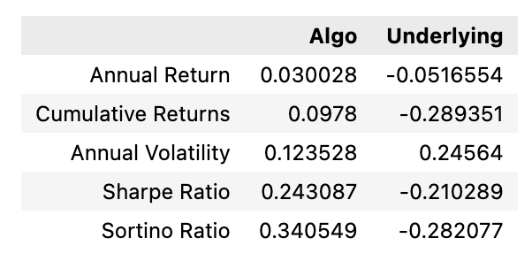
The provided Python code defines a function intended for evaluating the performance of an algorithmic trading strategy relative to the performance of a benchmark underlying asset. This function is used in the context of a project that examines the effectiveness of the Fama-French 3-Factor and 5-Factor Models in predicting portfolio returns.
The function, algo_vs_underlying, takes one argument, signals_df, which is likely a DataFrame containing trading signals and data necessary for evaluation. It defines a list of performance metrics such as Annual Return, Cumulative Returns, Annual Volatility, Sharpe Ratio, and Sortino Ratio that are of interest for assessing the trading strategy.
The function then constructs a new DataFrame with rows corresponding to these performance metrics and two columns designated for the algorithmic strategy Algo and the underlying benchmark asset Underlying. The evaluation results for both the algorithmic strategy and the underlying asset are calculated by presumably predefined functions, algo_evaluation and underlying_evaluation. The results from these evaluations for the respective Backtest data are populated into the new comparison DataFrame.
Finally, the comparison DataFrame is returned from the function, providing a side-by-side performance comparison that can be analyzed to determine how well the algorithmic strategy is doing in relation to just holding the underlying asset — commonly referred to as a Buy-and-Hold Strategy. The code is part of a larger algorithmic trading project that uses complex financial models for predictive purposes. In this context, the function enriches the analysis by offering a straightforward way to compare the trading strategy against a passive investment benchmark.
# Define function which accepts daily signals dataframe and returns evaluations of individual trades:
def trade_evaluation(signals_df):

  #initialize dataframe
  trade_evaluation_df = pd.DataFrame(
    columns=[
        'Entry Date',
        'Exit Date',
        'Shares',
        'Entry Share Price',
        'Exit Share Price',
        'Entry Portfolio Holding',
        'Exit Portfolio Holding',
        'Profit/Loss']
  )


  entry_date = ''
  exit_date = ''
  entry_portfolio_holding = 0
  exit_portfolio_holding = 0
  share_size = 0
  entry_share_price = 0
  exit_share_price = 0

  # Loop through signal DataFrame
  # If `Entry/Exit` is 1, set entry trade metrics
  # Else if `Entry/Exit` is -1, set exit trade metrics and calculate profit,
  # Then append the record to the trade evaluation DataFrame
  for index, row in signals_df.iterrows():
      if row['Entry/Exit'] == 1:
          entry_date = index
          entry_portfolio_holding = row['Portfolio Total']
          share_size = row['Entry/Exit Position']
          entry_share_price = row['Close']

      elif row['Entry/Exit'] == -1:
          exit_date = index
          exit_portfolio_holding = abs(row['Portfolio Total'])
          exit_share_price = row['Close']
          profit_loss = exit_portfolio_holding - entry_portfolio_holding
          trade_evaluation_df = trade_evaluation_df.append(
              {
                  'Entry Date': entry_date,
                  'Exit Date': exit_date,
                  'Shares': share_size,
                  'Entry Share Price': entry_share_price,
                  'Exit Share Price': exit_share_price,
                  'Entry Portfolio Holding': entry_portfolio_holding,
                  'Exit Portfolio Holding': exit_portfolio_holding,
                  'Profit/Loss': profit_loss
              },
              ignore_index=True)

  # Print the DataFrame
  return trade_evaluation_df
The Python code provided defines a function named trade_evaluation, which is part of an Algorithmic Trading project. The function is used to analyze trading signals within a given DataFrame that contains daily trading information, and it calculates a detailed performance evaluation for individual trades. The code begins by initializing a DataFrame to store the evaluation of trades with specific columns including dates for entry and exit, shares involved, share prices, the value of the portfolio holdings at entry and exit, and the profit or loss of the trade.
Within a loop, the function processes the signals DataFrame row by row. When a signal indicates an entry into a position denoted by Entry/Exit being 1, it records the date, portfolio value, number of shares traded, and entry share price. When a signal indicates an exit from a position denoted by Entry/Exit being -1, the corresponding exit date, portfolio value, and share price are recorded. It then calculates the profit or loss for that trade by comparing the entry and exit portfolio holdings.
After evaluating each trade, the function appends this information to the initialized DataFrame. Finally, once all rows have been processed and individual trades evaluated, the function returns the DataFrame, essentially providing a report of the trade performance according to the daily signals. Overall, this code serves to provide insights into the profitability of trades by pairing entry and exit points as per the strategy defined in the trading signals. It enables traders to assess each trades contribution to overall portfolio returns, which is useful for refining trading strategies based on models like the Fama-French 3-Factor or 5-Factor Model.
# Generate Evaluation table:
trade_evaluation_df=trade_evaluation(signals_df)
trade_evaluation_df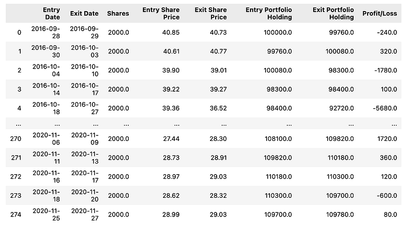
The Python code snippet provided appears to be part of a script used within an algorithmic trading project. Specifically, it relates to the evaluation of trading signals based on the Fama-French 3-Factor and 5-Factor models, which are used in finance to describe stock returns. The code is executing a function trade_evaluation which likely takes a DataFrame named signals_df as input.
This signals_df DataFrame probably contains trading signals that have been generated based on certain criteria from the Fama-French models. These signals could indicate potential buy or sell opportunities, depending on the strategy inherent to the models. Once the trade_evaluation function has processed this data, it outputs a new DataFrame assigned to the variable trade_evaluation_df. This resulting DataFrame is designed to systematically assess the performance of the trading signals. It may include metrics like return on investment, accuracy of signals, or other statistical measures that help determine the effectiveness of the trading signals produced by the Fama-French models.
The purpose of this code is to facilitate a rigorous evaluation of how well the trading strategy performs when applying the Fama-French factors to actual or hypothetical trades. Traders or portfolio managers can use the results to calibrate their models, improve their strategies, and ultimately make more informed investment decisions.
# Set X and y variables:
y = combined_df.loc[:, 'Returns']
X = combined_df.drop('Returns', axis=1)
X = X.drop('Close',axis=1)

# Add "Constant" column of "1s" to DataFrame to act as an intercept, using StatsModels:
X = sm.add_constant(X)

# Split into Training/Testing data:
split = int(0.8 * len(X))
X_train = X[: split]
X_test = X[split:]
y_train = y[: split]
y_test = y[split:]

# Run Ordinary Least Squares (OLS )Model:
model = sm.OLS(y_test, X_test)
model_results = model.fit()
print(model_results.summary())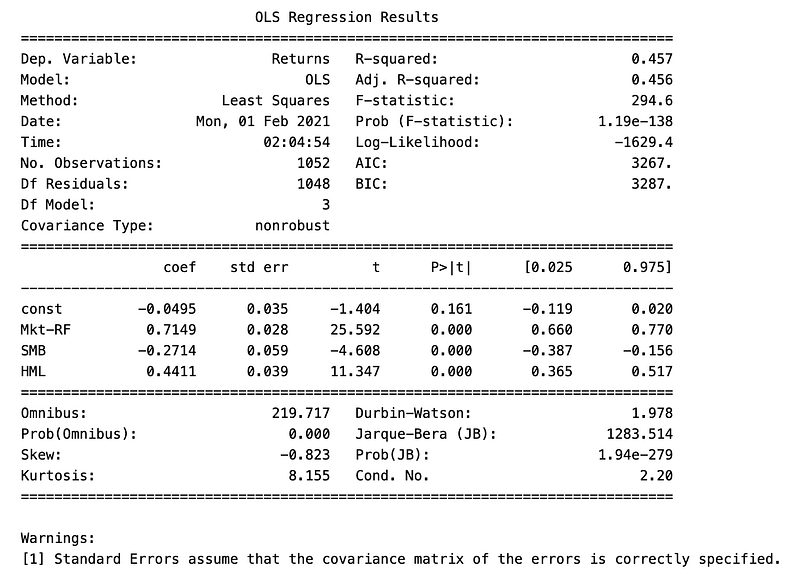
The provided Python code is part of an algorithmic trading project that utilizes the Fama-French 3-Factor and 5-Factor models to predict portfolio returns. The goal of this code is to prepare data for regression analysis, conduct the analysis, and report the results.
In the initial setup, the code defines the dependent variable y as the Returns column from a DataFrame named combined_df. Then, the code creates the independent variables X by excluding the Returns and Close columns from the same DataFrame. Next, the code inserts a column of ones to the independent variables DataFrame X to represent the intercept term for the regression model.
This is a requirement for performing statistical tests and interpreting the model accurately. Subsequently, the code divides the data into training and testing subsets. This split is usually done to train the model on a portion of the data in this case, 80% and to test its predictive power on the remaining unseen data. An Ordinary Least Squares OLS regression model is then fitted using the independent variables of the testing set X_test and the dependent variable of the testing set y_test.
Although typically, an OLS model is fit on the training set and evaluated on the test set, here it is directly applied to the test set. Upon fitting the model, the script generates a summary of the models results. This summary includes statistical measures that help evaluate the performance and significance of the individual factors involved in the model. The output of the model summary will guide the user on how well the factors explain the portfolios returns.
# Plot Partial Regression Plot:
fig = sm.graphics.plot_partregress_grid(model_results, fig = plt.figure(figsize=(12,8)))
plt.show()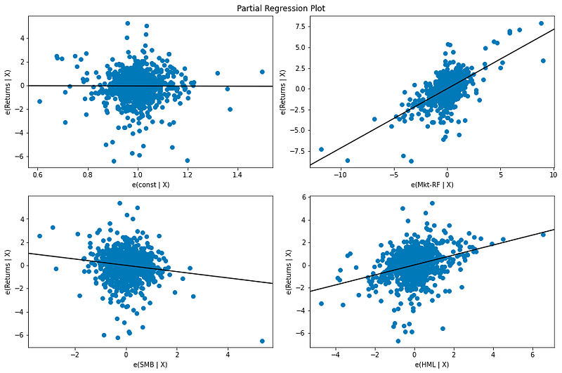
This Python code snippet is responsible for generating a partial regression plot for a statistical model, likely from the results of an econometric analysis examining the Fama-French 3-Factor or 5-Factor Model. The Fama-French models are used to explain stock returns, and this specific plot would be useful in an Algorithmic Trading project to visualize the relationship between portfolio returns and the factors included in the model, after accounting for the impact of other variables.
The function plot_partregress_grid from the statsmodels library sm.graphics takes the results of a regression model assumed to be stored in the variable model_results and plots the relationship between the dependent variable and each predictor variable, one at a time, while controlling for the other predictors. The fig parameter receives a new figure object plt.figure with a specified size, creating a space where the plots will be drawn.
Once the function has created the partial regression plot on the figure, the plt.show command is called to display the plot. This visual representation helps in understanding how much of the variation in portfolio returns can be attributed to each individual factor such as market risk, size, value, profitability, or investment while holding other factors constant, which is crucial for making informed trading decisions based on the Fama-French model analysis.
# Plot P&L Histrogram:
trade_evaluation_df["Profit/Loss"].hist(bins=20)
This Python code snippet is responsible for generating a histogram plot of the Profit/Loss values from a dataframe named trade_evaluation_df. A histogram is a graphical representation showing a visual impression of the distribution of the Profit/Loss data. The code creates a histogram with 20 bins, meaning that it will divide the range of Profit/Loss values into 20 intervals and count how many values fall into each interval.
The purpose of this code is to help visualize the performance of a trading algorithm as part of an Algorithmic Trading project. By plotting the profits and losses of trades, the histogram allows traders and analysts to quickly perceive the frequency and distribution of the trading outcomes, which can be essential in assessing the effectiveness of the trading strategies being evaluated.
The context of this code implies it is used to examine the Fama-French 3-Factor and 5-Factor Models, which are models that describe stock returns in terms of various risk factors. Histograms can be particularly useful in this kind of analysis, as they help to illustrate whether the models are predicting portfolio returns effectively by showing the distribution and range of the profits and losses that result from applying the algorithm based on these factors.
# Define function that plots Algo Cumulative Returns vs. Underlying Cumulative Returns:
def underlying_returns(signals_df):
  underlying=pd.DataFrame()
  underlying["Close"]=signals_df["Close"]
  underlying["Underlying Daily Returns"]=underlying["Close"].pct_change()
  underlying["Underlying Daily Returns"].fillna(0,inplace=True)
  underlying['Underlying Cumulative Returns']=(1 + underlying['Underlying Daily Returns']).cumprod() - 1
  underlying['Algo Cumulative Returns']=signals_df["Portfolio Cumulative Returns"]

  graph_df=underlying[["Underlying Cumulative Returns", "Algo Cumulative Returns"]]

  return graph_df
The provided Python code defines a function thats intended to facilitate the comparison between the cumulative returns of an algorithm-driven trading strategy and the underlying asset it is based on. The code does this by performing calculations on a dataframe presumably containing historical price data and trading signals.
The function first creates a new dataframe to store the underlying assets prices and calculates the daily returns by comparing the price changes from one day to the next. It replaces any missing values in the daily returns with zero to maintain continuity. From these daily returns, it then computes the cumulative returns, which represent the total return over time, accounting for the compounding effect. In parallel, the function retrieves the cumulative returns of the trading algorithm, presumably already calculated within the signals dataframe.
This allows for a like-for-like comparison. Finally, the function prepares a new dataframe containing only the cumulative returns of both the underlying asset and the trading algorithm. This resultant dataframe is structured for easy visualization, such as plotting the returns over time to compare the performance of the algorithm against the underlying assets performance.
The purpose of this code is as part of an assessment of the Fama-French models in predicting portfolio returns within an algorithmic trading project. The visual comparison facilitated by this function can be critical in understanding the efficacy of the algorithm in capturing various risk factors and delivering excess returns over the asset it trades on.
# Generate Cumulative Return plot using above defined function:
underlying_returns(signals_df).plot(figsize=(20,10))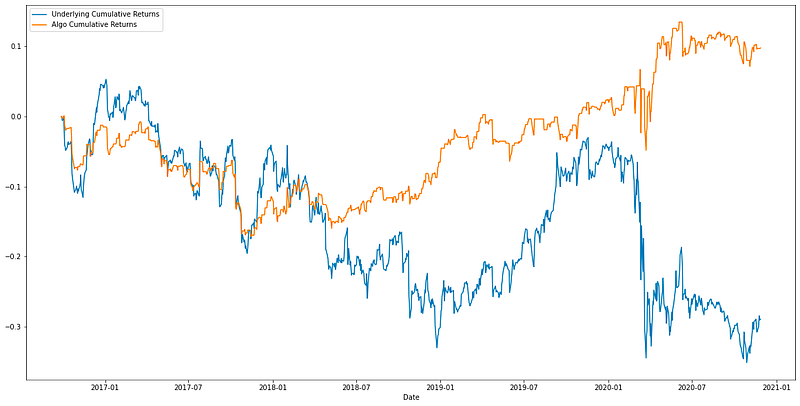
The given Python code snippet is part of a larger project that applies algorithmic trading concepts, particularly dealing with the Fama-French 3-Factor and 5-Factor Models used to explain stock returns. These models are well-known in financial economics and are used to describe the impact of various risk factors on the returns of a portfolio. Specifically, the code is generating a plot of the cumulative returns of a trading strategy or a portfolio.
This is accomplished by calling a function underlying_returns with signals_df as its parameter, which presumably calculates the returns based on trading signals or investment decisions contained within the signals_df dataframe. The result of this function is a series of cumulative returns over time. Once the returns are calculated, the code then proceeds to plot these cumulative returns using the plot function, which is a part of pandas or matplotlib libraries in Python.
The plot is configured to have a figure size of 20x10 inches, which specifies the width and height of the plot for visualization purposes. By analyzing such a plot, investors and analysts can visually assess the performance of their trading strategies over time, helping to make informed decisions regarding the efficacy of applying the Fama-French models in predicting portfolio returns.
This Is not the complete code, find the entire code here:


