Hands-on Introduction to Hidden Markov Model

What is a Hidden Markov Model (HMM) and how to build one in Python.

First thing first, what is a Markov Model? Imagine the following scenario: you want to know whether the weather tomorrow will be sunny or rainy. From your experience, the probability of tomorrow being sunny is 90% if at present the weather is also sunny. But if it is currently raining, then the probability of tomorrow being sunny is lower at 50% chance. This collection of scenario can be described as a Markov process.

If you are unfamiliar with Markov process, do read this introductory post below.

Hidden Markov Model

Before we go straight into formalizing Hidden Markov Model (HMM), let’s define our running example using the weather scenario above.

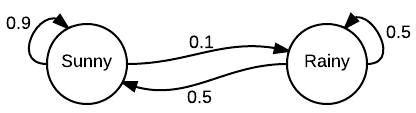
with the following transition matrix, T.

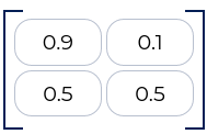
• 1st row: probability from sunny to sunny is 0.9 | probability from sunny to rainy is 0.1
• 2nd row: probability from rainy to sunny is 0.5 | probability from rainy to rainy is 0.5

But now suppose, for some reason, you can’t determine the current weather. Perhaps you are quarantined in an isolation room without any window to peek through. Nevertheless, you can still feel the temperature from your isolation room to either be cold or hot.

This is called Hidden Markov: the cold and hot states are the visible Markov, while the sunny and rainy states are the invisible Markov processes, and each hidden state generates a random temperature observations to us.

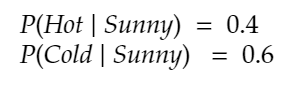
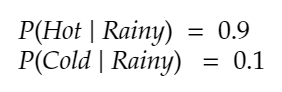
Also, suppose we observe the following conditional probabilities:

• Conditional probabilities of a 1) hot or 2) cold temperature given a hidden sunny day

• Conditional probabilities of a 1) hot or 2) cold temperature given a hidden rainy day

So what can we do with all these information? Let’s ask a simple question.

Basic Worked Example

If in the past 2 days the temperature has been consistently, what is the most likely sequence of weather (hidden to us)?

In these 2 days, there are 2 (temperatures) * 2 (weather) = 4 variations for the underlying Markov options: (Sunny, Rainy), (Rainy, Sunny), (Sunny, Sunny), or (Rainy, Rainy).

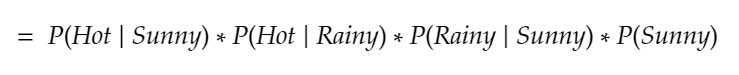
To calculate the probability, we need to sum up all 4 of these variations. But for now, let us use one option (Sunny, Rainy) to illustrate how HMM can be computed.

1. Using the Bayesian statistical formula:

2. Further breaking down:

3. Filling in the numbers with our prior probabilities (where P(Sunny) is a prior knowledge with probability 0.5):

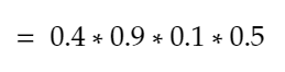
Hence, given 2 days of observable hot temperature, the probability of the hidden weather being (Sunny then Rainy) is 0.018. Pretty low!

However, a brute force solution like this could easily take an exponential running time complexity. Imagine if you are now given 10 different temperature observations and are asked to predict the most likely sequence of hidden weather events. Using this brute force algorithm would pose a headache.

Do we then have more efficient HMM algorithm? Introducing the Viterbi Algorithm.

Viterbi Algorithm: Finding Hidden States

Viterbi algorithm is defined by a sequence of observations o₁,…,oₜ and for each of the state i, and time into the future t=1,…,T, we define

This looks daunting! Let me try to explain this in plain English. Essentially, Viterbi attempts to find the best path that explains the current observation.

Viterbi in Plain English

Suppose you want to know the probability of a sequence of weather (hidden state) given 2 consecutive temperature observations (eg. Hot then Hot). Computing the probability for the next day would require you to consider 2 possible states (hot and cold), and the day after that 4 possible states. You can straight away notice the exponential complexity of this branching method if you are running the algorithm for a substantially large t.

But soon you realize that the probability of a state on t day, doesn’t depend on the probability of the third or fourth or fifth day. It only depends on the probability of the day before (ie. t-1 day). Following that logic, you can aggregate current (and by extension, previous) state probabilities to produce a distribution describing 2 states, as opposed to 4. This is then performed recursively (t number of times) to find the state (and path) with the highest probability as what the Viterbi Algorithm produces.

Viterbi in Python

Let’s try to write a Viterbi program to further illustrate how the algorithm works. We are going to estimate the likeliest sequence of 13 hidden weather states given a sequence of 14 temperature observations (including the present observation).

1. First, we initialize our states and observations

import numpy as np
import pandas as pd

obs_map = {'Cold':0, 'Hot':1}
obs = np.array([1,1,0,1,0,0,1,0,1,1,0,0,0,1])

inv_obs_map = dict((v,k) for k, v in obs_map.items())
obs_seq = [inv_obs_map[v] for v in list(obs)]

obs_seq
>>> ['Hot','Hot',...,'Cold','Hot']

2. And our initial probability matrices

• for the hidden states…

hidden_states = ['Sunny', 'Rainy']
h_pr = [0.5, 0.5]
state_space = pd.Series(h_pr, index=hidden_states, name='states')

hmm_df = pd.DataFrame(columns=hidden_states, index=hidden_states)
hmm_df.loc[hidden_states[0]] = [0.9, 0.1] #Sunny
hmm_df.loc[hidden_states[1]] = [0.5, 0.5] #Rainy

hmm_val = hmm_df.values

hmm_df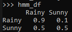

• and the observable states…

i_pr = [0.6, 0.4] # initial probabilities vector
obs_states= ['Cold', 'Hot']

obs_df = pd.DataFrame(columns=obs_states, index=hidden_states)
obs_df.loc[hidden_states[0]] = [0.6,0.4] #Sunny
obs_df.loc[hidden_states[1]] = [0.1,0.9] #Rainy

obs_val = obs_df.values

obs_df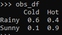

3. Now the last part is to implement the recursive Viterbi function as defined above.

When running the program

path, delta, phi = viterbi(h_pr, hmm_val, obs_val, obs)

we get the following output.

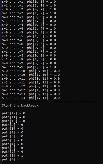
So, the likely sequence of the hidden weather states given our sequence of temperature observations is: Rainy (1), Rainy (1), Sunny (0), …, Sunny (0).

Parting Thoughts

So that’s it for our introduction to HMM which attempts to find the likeliest sequence of hidden states given a set of observations using the Viterbi algorithm. There’s a second algorithm that is called the Baum-Welch model. It leverages on learnable parameters that best fit the HMM model. Although this is beyond the scope of this post, you can find a good introduction here.

I regularly summarize AI research papers in plain English and beautiful visualization via my Email Newsletter, do subscribe at https://tinyurl.com/2npw2fnz.