Handling Shocks in Time Series Forecasting: A Comparison of Strategies Using Facebook’s Prophet

Exploring Different Approaches to Incorporate Shocks like Covid-19 in Time Series Forecasting with Prophet and Evaluating Their Performance Using the Mean Average Percentage Error (MAPE).

This is my first article ever — so don’t judge me too hard ;-)

I recently discovered that Facebook tackled the topic of shock handling within their documentation of Prophet: you can find it here.

A few words about Prophet before we start: Prophet is a forecasting procedure developed by Facebook that uses time series data to forecast future values. It is an open-source software package written in Python and R and is designed to be easy to use, accurate, and scalable. According to my research (looking at GitHub stars), it is the most used forecasting library in the industry.

Quick summary of their case study: Taking the open data about the number of pedestrians by hour provided by the city of Melbourne, Facebook presents different strategies for how to incorporate shocks like Covid 19 into the Prophet model. Two different strategies are introduced in detail: 1. no adjustments at all and 2. treating COVID-19 lockdowns as one-off holidays.

Both approaches are analyzed visually with no objective evaluation method. Furthermore, only in-sample analyses were conducted which always has a high risk of overfitting the data. It is mentioned in the end, that there are more strategies.

In the following, I will present four different strategies to handle shock events. For that, I will split the dataset into train and test sets (out-of-sample analysis) and evaluate the model performance with the MAPE score (Mean Average Percentage Error). MAPE is a common metric used to measure the accuracy of a forecasting model by calculating the average percentage difference between actual and predicted values. By that, we will know which method works best for this concrete case study.

These are the four strategies:

1. No adjustment
2. Treating COVID-19 lockdowns as a one-off holidays
3. Deleting COVID-19 lockdown periods from the training set
4. Adding the Corona Stringency Index as a regressor

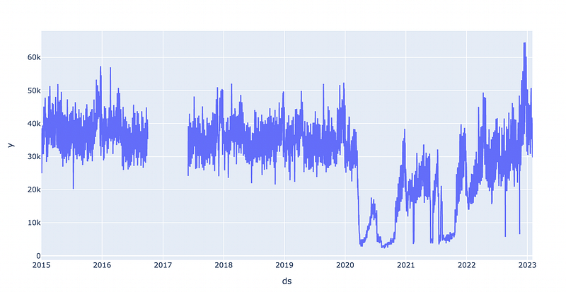
The data:

We will use the same data as Facebook does in the example in the linked case study. However, I updated the dataset and got data until the end of January 2023.

As you can see in the graph below, we have some missing data for 2016/2017. That does not matter because the dataset is still big enough. In the years 2020 and 2021, we can see dips due to Covid 19.

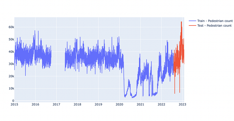
Splitting the data

As mentioned above, we split the dataset into train and test sets. Usually, in machine learning, you would draw a random split. In time series forecasting, we need to keep the time component in mind. Therefore, I decided to pick a concrete cutoff date to split the data. The data will be split by August 2022 so that we have exactly 6 months of test data. I could have picked any other date, the choice was random. Another (probably better) approach would be to evaluate with sliding windows. However, for simplicity, we will stick to the fixed cutoff date.

split_date = ‘2022–08–01’

train = df_mc[df_mc.ds < pd.to_datetime(split_date, format=’%Y-%m-%d’)]
test = df_mc[df_mc.ds >= pd.to_datetime(split_date, format=’%Y-%m-%d’)]

Below you can see the split data: blue will be used to train the model, and red will be used to evaluate the performance.

Now, we can test the four strategies:

1. No adjustment

Exactly as in the documentation, we will try the model with no adjustments at all:

m = Prophet()
m = m.fit(train)
# exactly 184 days between begin of August and end of January 
future = m.make_future_dataframe(periods=184)
forecast = m.predict(future)

Now, we have the prophet predictions until the end of January in the forecast variable. Before calculating the MAPE score, there are still two issues to solve. First of all, the test set contains 4 NaN rows with missing data. Secondly, the forecast variable holds also the predictions for the past data (since 2015).

To get rid of the previous dates and the missing data, we will inner join the forecast with the test data and in the next step remove rows where the test data is missing.

ev = test.merge(forecast, on='ds')[['ds','y','yhat']]
ev=ev.dropna(axis=0)

In the next step, we can easily calculate the MAPE score:

from sklearn.metrics import mean_absolute_percentage_error
mean_absolute_percentage_error(ev['y'],ev['yhat'])

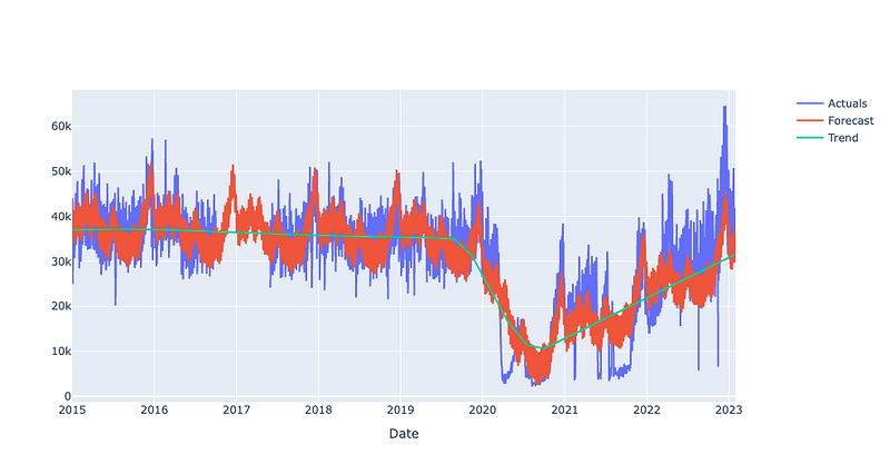
# MAPE:0.20834926453080485

So, our benchmark is 0.2083.

Let’s have a quick look at the model: it correctly detects the lockdown periods as the trend changes. However, as we can see, the overlap of actuals and forecasts is weak for the final months.

2. Treating COVID-19 lockdowns as one-off holidays

Here, we define custom one-off ‘holidays’. In Prophet, custom holidays allow the user to specify dates and/or ranges of dates that are known to have an impact on the time series being analyzed. By including custom holidays, the model can account for the effect of these events in its forecasts, which can lead to more accurate predictions. However, anything can be defined as a custom holiday. For example, in the documentation, Superbowl days are defined as holidays.

If you want to know more about the concept of holidays in prophet, I can recommend reading through the documentation.

lockdowns = pd.DataFrame([
    {'holiday': 'lockdown_1', 'ds': '2020-03-21', 'lower_window': 0, 'ds_upper': '2020-06-06'},
    {'holiday': 'lockdown_2', 'ds': '2020-07-09', 'lower_window': 0, 'ds_upper': '2020-10-27'},
    {'holiday': 'lockdown_3', 'ds': '2021-02-13', 'lower_window': 0, 'ds_upper': '2021-02-17'},
    {'holiday': 'lockdown_4', 'ds': '2021-05-28', 'lower_window': 0, 'ds_upper': '2021-06-10'},
    {'holiday': 'lockdown_5', 'ds': '2021-07-16', 'lower_window': 0, 'ds_upper': '2021-10-21'},
])
for t_col in ['ds', 'ds_upper']:
    lockdowns[t_col] = pd.to_datetime(lockdowns[t_col])
lockdowns['upper_window'] = (lockdowns['ds_upper'] - lockdowns['ds']).dt.days

Afterward, we also need to pass the lockdown variable to Prophet and then can calculate the forecast as before:

m2 = Prophet(holidays=lockdowns)
m2 = m2.fit(train)
future2 = m2.make_future_dataframe(periods=184)
forecast2 = m2.predict(future2)

The evaluation step is exactly as before:

ev2 = test.merge(forecast2, on='ds')[['ds','y','yhat']]
ev2=ev2.dropna(axis=0)

mean_absolute_percentage_error(ev2['y'],ev2['yhat'])
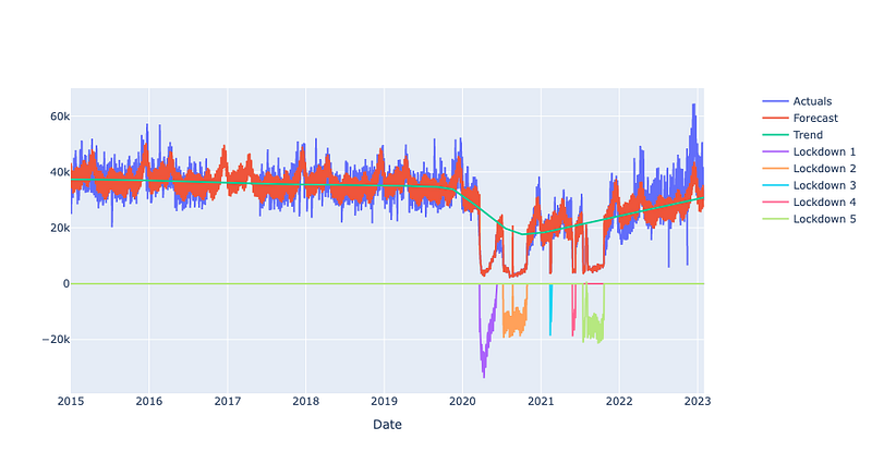
# MAPE:0.20377607223879712

And as we can see, the MAPE slightly decreased. Conclusion: Using the lockdowns as holidays works better than doing nothing.

Finally, let’s have a look at the graph again. As we can see, the lockdown periods are now perfectly captured by the model. However, that is not relevant for a future forecast. For the time since begin of 2022, linear growth with no further trend changes is predicted.

3. Deleting COVID-19 lockdown periods from the training set

Another strategy is simply deleting ‘weird’ data. This only works if we have enough data history. In this case, we should be fine.

Since we now change the data frame, first of all, we need to make a copy:

train_del = train.copy()

In the next step, we delete the same periods that we defined as lockdowns in the previous strategy.

# delete rows between dates X and Y in df
def del_date_range(df, startdate, enddate = None):
    if enddate == None:
        df.loc[df.ds == startdate, 'y'] = None
    else:
        df.loc[(df.ds >= startdate) & (df.ds <= enddate), 'y'] = None 
    return df

train_del = del_date_range(train_del,'2020-03-21','2020-06-06')
train_del = del_date_range(train_del,'2020-07-09','2020-10-27')
train_del = del_date_range(train_del,'2021-02-13','2021-02-17')
train_del = del_date_range(train_del,'2021-05-28','2021-06-10')
train_del = del_date_range(train_del,'2021-07-16','2021-10-21')

We already know the next steps by heart:

m3 = Prophet()
m3 = m3.fit(train_del)
future3 = m3.make_future_dataframe(periods=184)
forecast3 = m3.predict(future3)

ev3 = test.merge(forecast3, on='ds')[['ds','y','yhat']]
ev3=ev3.dropna(axis=0)
mean_absolute_percentage_error(ev3['y'],ev3['yhat'])
# MAPE:0.1991013184824403

The best result so far! Deleting data works better than setting custom holidays in this use case.

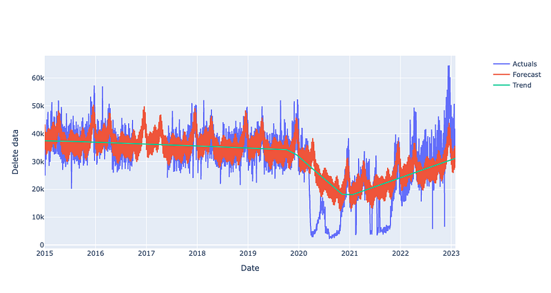
A quick look at the graph: the lockdown periods are now not captured at all — that is not a surprise, we did not give the dips to the model at all. For the time since 2021, we again predict linear growth with no change points here.

4. Adding the Corona Stringency Index as a regressor

The corona stringency index (short: CSI) is a index created by the Oxford Coronavirus Government Response Tracker (OxCGRT) project.

The stringency index is a composite measure based on nine response indicators including school closures, workplace closures, and travel bans, rescaled to a value from 0 to 100. A higher score indicates a stricter response (i.e. 100 = strictest response). If policies vary at the subnational level, the index is shown as the response level of the strictest sub-region.

You can find more information (and the data) here: https://ourworldindata.org/covid-stringency-index

First of all, we need to prepare the data. We take the CSV, filter on data for Australia only, and keep only the two relevant columns: date and the index.

# source https://ourworldindata.org/covid-deaths
csi = pd.read_csv("owid-covid-data.csv") # took the csv from the webpage 
csi = csi.loc[csi.iso_code == 'AUS', ['date','stringency_index']]
csi.date = pd.to_datetime(csi.date)
csi.fillna(0,inplace=True)

In the next step, we are going to take a copy of the train data and add the CSI data to it:

train_csi = train.copy()
train_csi = train_csi.merge(csi,how=’left’, left_on=’ds’, right_on=’date’)[[‘ds’,’y’, ‘stringency_index’]]
train_csi[‘stringency_index’].fillna(0,inplace=True)

Afterward, we run the prediction similar to the three times before but we apply three changes now. 1. The new regressor has to be added after initializing the model, 2. we take the just created train set with the CSI data and 3. we also add the CSI to the future dates.

m4 = Prophet()
m4.add_regressor('stringency_index')
m4 = m4.fit(train_csi)

future4 = m4.make_future_dataframe(periods=184)

future4 = future4.merge(csi,how='left', left_on='ds', right_on='date')[['ds','stringency_index']]
future4['stringency_index'].fillna(0,inplace=True)
forecast4 = m4.predict(future4)

The last evaluation for today:

ev4 = test.merge(forecast4, on='ds')[['ds','y','yhat']]
ev4=ev4.dropna(axis=0)
mean_absolute_percentage_error(ev4['y'],ev4['yhat'])
# MAPE: 0.1916578295110247

And we have a winner! Applying the CSI lead to the lowest MAPE score among the strategies!

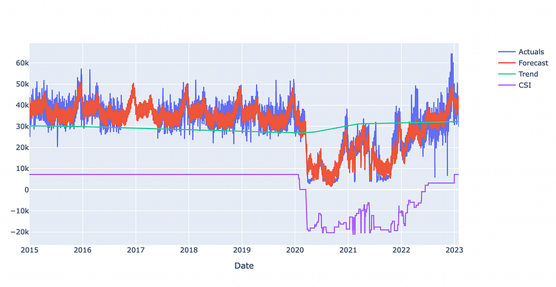
Let’s check the last graph: the lockdown periods are fairly well detected. The trend for the future is only slightly positive (in comparison to all previous methods). That trend is closer to the one that we had in the pre-corona time.

Final words

The fourth strategy works best in this case. I have already tried the different approaches with other data sets where deleting data leads to the best results. So, keep in mind that there is no general answer for all use cases. Also, I did not apply any tuning techniques here: E.g. allowing prophet to find more trend change points could probably lead to a better result with no further adjustments (however, it could also lead to overfitting).

I hope you enjoyed my very first article. There might be more soon!