[ML Shot of the Day]: Discretization of Continuous Attributes

Handling Continuous features in Decision Trees

Choosing the optimal splitting point for continuous attributes in Decision Trees

A Crash Course on Decision Trees and Splitting Measures:

• Decision Trees and its variants, Random Forests, XGBoost, CatBoost are popularly used in the Machine Learning world (including competitions).
• Training a Decision Tree for a classification problem involves recursively splitting the data into smaller subsets until each node contains data belonging to a single class.
• Different measures (Information Gain, Gini Index, Gain ratio) are used for determining the best possible split at each node of the decision tree.

Splitting Measures for growing Decision Trees:

• Recursively growing a tree involves selecting an attribute and a test condition that divides the data at a given node into smaller but pure subsets.
• The measures used for determining the best split computes the degree of impurity of the child nodes.
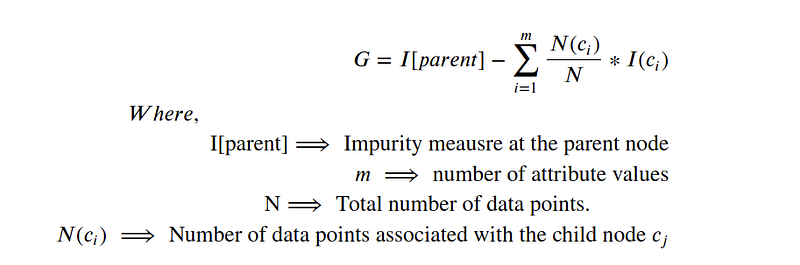
• Computing the impurity of child nodes with respect to that of parent nodes is called Gain. Higher the Gain (G), the better the split.
• Let pₖ be the proportion of records belonging to class k at a given node. The impurity measures are given by :

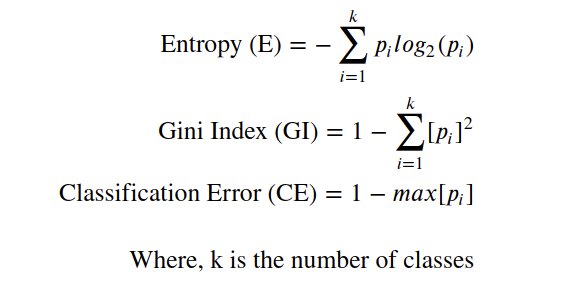
• The Gain is computed as:

The curious case of Continuous Attributes:

It can be seen that the computation of splitting measures assumes finite (read: discrete) attribute values. This begs the question, How are continuous-valued attributes handled in decision trees?

Take some time to think about it (Not long though..its an ML shot)

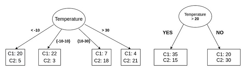
The test condition for a continuous-valued attribute can either be expressed using a comparison operator (≥, ≤) or the attribute can be split into a finite set of range buckets. It is important to note that a comparison-based test condition gives us a binary split whereas range buckets give us a multiway split.

Converting a continuous-valued attribute into a categorical attribute (multiway split) :

• An equal width approach converts the continuous data points into n categories each of equal width. For instance, a continuous-valued attribute with a range of 0–50 can be converted into 5 categories of equal width -[0–10), [10–20), [20–30), [30–40), [40–50]. The number of categories is a hyper-parameter.
• It is important to note that the equal width approach is sensitive to outliers.
• The equal frequency approach converts the continuous-valued attribute into n categories such that each category contains approximately the same number of data points.
• More sophisticated methods involve the use of unsupervised clustering algorithms to define the optimal categories.

Converting a continuous-valued attribute into a binary attribute (two-way split):

• A comparison bases test condition of the form attribute >= v involves the determination of v.
• It is easy to see that a brute force approach of trying out every single value of the continuous variable is computationally expensive.
• A better way for identifying the split candidates involves sorting the values of the continuous attribute and taking the midpoint of the adjacent values in the sorted array.
• As seen in the figure below, the potential candidates for the split can be narrowed down to -15, -9, 0, 12, and 21.

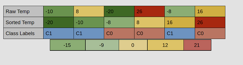
• It is evident that the number of candidates after taking the midpoint of the sorted array can still be computationally expensive.
• A more optimized version involves selecting midpoint candidates with different class labels. This will narrow down the candidates to -9 and 12 which is a significant improvement over the brute force approach.

Final Thoughts:

• The field of AI/ML/DS is evolving at an incredible pace. The goal of ML shots is to cover some of the tricky concepts that are often ignored.
• Do reach out to me if you have ideas for ML shots.

Let’s have a chat :

Reach out to me on Linkedin to brainstorm ideas.