Guide to L1 and L2 regularization in Deep Learning

Alternative Title: understand regularization in minutes for effective deep learning. All about regularization in Deep Learning and AI

Regularizations prevents model overfitting by restricting parameter freedom. This is a beginner friendly regularization formula deep dive. We write beginner friendly tutorials: Softmax, Natural Language Processing, Cross Entropy Loss and GPT-3 model strengths and GPT-3 weakness.

Read the full disclaimer, basically our tutorials are for educational purpose only. We are NOT responsible for any commercial, production use nor do we advise it. All articles are exclusively published on our Medium and subdomains. No repost, no scraping. Thanks.

We will discuss regularization methods used to restrict weights. By restricting the growth of weights, the model becomes easier to compute and better at generalizing. (Regularization puts pressure on weights prevent weights from growing out of control.) By generalizing well, we mean the model should perform well on training data as well as new inputs — unseen data. It practically is the holy grail of machine learning. The senior technical manager we interviewed, states, help algorithms generalize well is a key goal in his work.

There are quite a few regularization methods, we are only covering the two popular ones L1 and L2 regularization.

Related concepts include: bias, variance, underfitting and overfitting. High bias and underfitting means our model or algorithms is not sophisticated enough, or not the right fit for capturing the pattern of the data. Overfitting, means the model or algorithms is making unnecessarily complex proximation to mimic the pattern of the data that may be more memorization than learning the real pattern. For example, if a dataset can be simply fitted with line, using a polynomial line that bends around each datapoint makes the model overfit, and does not generalize well to unseen data.

Regularization helps us reduce test error (holdout dataset) and generalize better. It does not necessarily reduce training error. It achieves the goal by adding or modifying weights and terms in the objective function aka cost function, loss function. The choice of regularization will have effects on the learned weights and behavior pattern of the weights.

This year 2021 we are launching a new machine learning for beginners course to help you make learning machine learning your new year resolution. Paid members get personalized learning journey, weekly lessons in their inbox, code snippets, cheat sheets, infographics, even technical interview tips, and easter eggs and perks. Sign up to join our early beta program at a reduced price. [email protected] Pilot course launching Q1 2021. The course organize basic machine learning concepts into cohesive smart, searchable posts. You won’t have to google around to learn important concepts.

Have a question about this tutorial? Need additional help? Message us on our LTC app.

“An effective regularizer is one that makes a profitable trade, reducing variance significantly while not overly increasing the bias.” Goodfellow et al.

In neural networks, linear regression, logistic regression, a simple yet effective regularization strategy can be adding a penalty term to loss function. The penalty term can have a hyperparameter that controls the rate of change. The extra term must be dependent on theta or the weight parameter, else it won’t affect the objective function.

To put it simply the new cost function looks like:

loss_function(weight, input_data) = loss_function(weight, input_data) + rate * penalty(weight)

# another way to write the formula

loss_function(weight, input_data) += rate * penalty(weight)

In plain English: loss function now equals to the old loss function plus the multiplication of rate and penalty. Pro tip the penalty term is a function of weight parameters. As weight w varies, the penalty term also varies. That’s the point. That’s why adding the penalty in loss function helps restrict the weights.

Below is the mathematical formula. The original loss function is represented by Greek letter J. The extra penalty term associated with regularization is denoted with Omega. Theta is the weight w. Alpha the rate of penalty.

Thanks to the interdisciplinary nature of machine learning, we often seen different symbols that have originated from other disciplines such as math, statistics, even Physics. Sometimes the symbols get confusing. You might be familiar with the loss function J if you took Andrew Ng’s academic Coursera class, but would not have seen it in practical Udacity nanodegrees that use Pytorch and Python so the loss function is readable variable loss= .

LIKE what you read? Support us by clapping for this article. Thank you!

How to Calculate the L2 Regularization Loss Function — Ridge Regression

L2 Ridge and L1 are probably the two most well known regularization.

In our premium course we will spend more time breaking down the math but here’s an overview of L2.

This year 2021 we are launching a new machine learning for beginners course to help you make learning machine learning your new year resolution. Paid members get personalized learning journey, weekly lessons in their inbox, code snippets, cheat sheets, infographics, even technical interview tips, and easter eggs and perks. Sign up to join our early beta program at a reduced price. [email protected] Pilot course launching Jan 2021. The course organize basic machine learning concepts into cohesive smart, searchable posts. You won’t have to google around to learn important concepts.

L2 parameter norm penalty commonly known as weight decay. This regularization strategy drives the weights closer to the origin — Goodfellow et al.

While the nomenclature ridge is hard to remember, L2 is an easy one. 2 refers to squared, x to the 2nd power, 2nd exponential.

def sumof_squared(weights):
    result = 0
    for w in weights:
        result += w*w
    return result

Above is the detailed pseudo code. Below is more abstracted.

#pseudo code

def penalty(weights):
    sum(squared(weights))

loss_function(weights, input_data) += rate/2 * penalty(weights)

The penalty on weights when using L2 regularization can increase quickly. Because the weight is squared. See above for Ian Goodfellow’s explanation of the behavior.

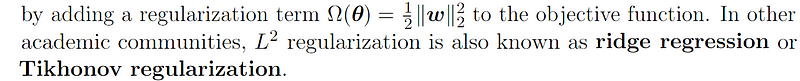
Again, here’s the math formula as seen in Ian Goodfellow’s Deep Learning textbook. It’s a dense read for newcomers, but we highly recommend it.

Omega is written as L2 norm of weight w, divided by 2. Pro tip : the 1/2 cancels out the 2nd power nicely when it is brought down in gradient, derivative calculations. Example squared(x), derivative is 2x. 2x / 2 = x. Just some nice math trick, which does not change the final result. The |||| double bars are called norms, also represent magnitude.

As machine learning practitioners, not researchers, we just need to know regularization adds penalty to weights in the loss function. And depends on the penalty mechanism, the behavior of optimization can have different results. By studying how optimized weights change with the penalty and its rate, and the original loss function which depends on weight, researchers have concluded the effectiveness of L2 regularization to help : “L2 regularization causes the learning algorithm to “perceive” the input X as having higher variance, which makes it shrink the weights on features whose covariance with the output target is low compared to this added variance.”.

You might have seen regularizations presented in contour graphs. We will explain more about how to read it in our course.

Have questions about this post? Paid members can leave a message and get answers.

Have a question about this tutorial? Need additional help? Message us on our LTC app.

How to calculate L1 Regularization and Loss Function

The other famous regularization method uses L1 calculation — absolute value. You can see the formula for penalty, regularization term aka Omega below is represented by the L1 norm, double bar with subscript of 1, or the sum of absolute values of weight.

#pseudo code
def sumof_abs(weights):
    result = 0
    for w in weights:
        result += abs(w)
    return result

Above is the detailed pseudo code. Below is more abstracted.

# pseudo code:

def penalty(weights):
    sum(abs(weights))

loss_function(weights, input_data) += rate * penalty(weights)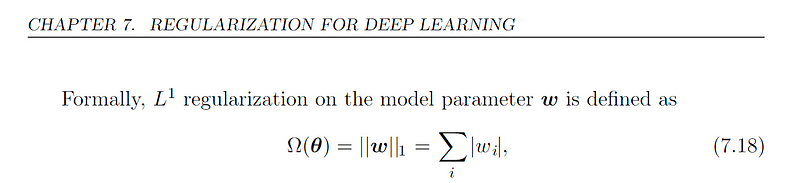

It’s easier to calculate rate of change, gradient for squared function than absolute penalty function, which adds nonlinearity to the loss function.

Intuitively when we think about absolute function, we can see that there is a distinct behavior change when the input is positive or negative. There’s a sharp angle where the output of absolute function becomes mirror image.

Similarly the L1 Regularization has behavior change when the weight is below equal to or above a particular threshold, determined by the rate and a mathematical matrix.

Mathematicians and researchers found that L1 regularizations when the weight is below the threshold, L1 regularization pushes all the weight values close to zero and thus result in sparse weight matrix. In plain English, some weights (coefficients) will be considered optimal at zero. If those features are columns of data, essentially these columns of data will be useless and won’t affect our final prediction. Sign up for our premium beginner’s ML course to learn more about how L1 Regularization can be used effectively in the data preprocessing step of machine learning workflow. In which we will also explain LASSO regularization.

Have a question about this tutorial? Need additional help? Message us on our LTC app.

Remember the high level takeaway is regularization just adds penalties to loss function. Both the loss function and penalty depends on the weight parameter, which machine learning algorithms use optimizer and gradient calculation to learn and optimize. Regularization operates on the loss function and weights. Research seems to indicate regularizations works in practice, helps models generalize better.

The rate parameter usually represented using greek letter lambda, which ranges between 0 and 1 {0, 1}. It’s an important hyperparameter. Some algorithms support min_lambda.