GRL Series

Graph Attention Networks Under the Hood

A Step-by-step Guide From Math to NumPy

Graph Attention Networks Layer —Image from Petar Veličković

Graph Neural Networks (GNNs) have emerged as the standard toolbox to learn from graph data. GNNs are able to drive improvements for high-impact problems in different fields, such as content recommendation or drug discovery. Unlike other types of data such as images, learning from graph data requires specific methods. As defined by Michael Bronstein:

[..] these methods are based on some form of message passing on the graph allowing different nodes to exchange information.

For accomplishing specific tasks on graphs (node classification, link prediction, etc.), a GNN layer computes the node and the edge representations through the so-called recursive neighborhood diffusion (or message passing). According to this principle, each graph node receives and aggregates features from its neighbors in order to represent the local graph structure: different types of GNN layers perform diverse aggregation strategies.

The simplest formulations of the GNN layer, such as Graph Convolutional Networks (GCNs) or GraphSage, execute an isotropic aggregation, where each neighbor contributes equally to update the representation of the central node. This blog post is dedicated to the analysis of Graph Attention Networks (GATs), which define an anisotropy operation in the recursive neighborhood diffusion. Exploiting the anisotropy paradigm, the learning capacity is improved by the attention mechanism, which assigns different importance to each neighbor's contribution.

If you are completely new to GNNs and related concepts, I invite you to read the following introductory article:

Understanding the Building Blocks of Graph Neural Networks (Intro)

An intuition (with running code) on the framework to analyze and learning graph data with neural architectures

towardsdatascience.com

GCN vs GAT — Math Warm-Up

This warm-up is based on the GAT details reported by the Deep Graph Library website.

Before understanding the GAT layer's behavior, let’s recap the math behind the aggregation performed by the GCN layer.

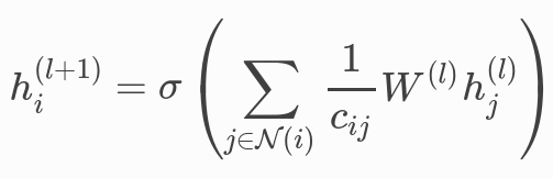
N is the set of the one-hop neighbors of node i. This node could also be included among the neighbors by adding a self-loop.
c is a normalization constant based on the graph structure, which defines an isotropic average computation.
σ is an activation function, which introduces non-linearity in the transformation.
W is the weight matrix of learnable parameters adopted for feature transformation.

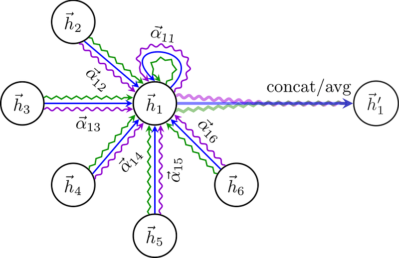
The GAT layer expands the basic aggregation function of the GCN layer, assigning different importance to each edge through the attention coefficients.

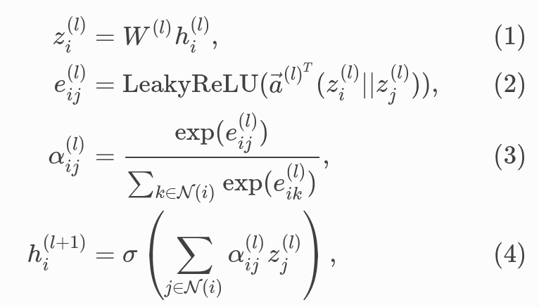
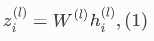
Equation (1) is a linear transformation of the lower layer embedding h_i, and W is its learnable weight matrix. This transformation helps achieve a sufficient expressive power to transform the input features into high-level and dense features.
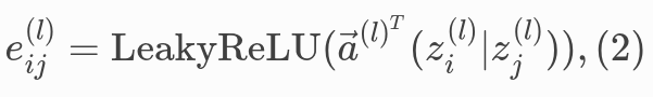
Equation (2) computes a pair-wise un-normalized attention score between two neighbors. Here, it first concatenates the z embeddings of the two nodes, where || denotes concatenation. Then, it takes a dot product of such concatenation and a learnable weight vector a. In the end, a LeakyReLU is applied to the result of the dot product. The attention score indicates the importance of a neighbor node in the message passing framework.
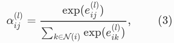
Equation (3) applies a softmax to normalize the attention scores on each node’s incoming edges. The softmax encodes the output of the previous step in a probability distribution. As a consequence, the attention scores are much more comparable across different nodes.
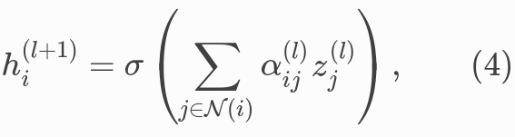
Equation (4) is similar to the GCN aggregation (see the equation at the beginning of the section). The embeddings from neighbors are aggregated together, scaled by the attention scores. The main consequence of this scaling process is to learn a different contribution from each neighborhood node.

NumPy Implementation

The first step is to prepare the ingredients (matrices) to represent a simple graph and perform the linear transformation.

NumPy code

Output

----- One-hot vector representation of nodes. Shape(n,n)

[[0 0 1 0 0] # node 1
 [0 1 0 0 0] # node 2
 [0 0 0 0 1]
 [1 0 0 0 0]
 [0 0 0 1 0]]

----- Embedding dimension

----- Weight Matrix. Shape(emb, n)

[[-0.4294049   0.57624235 -0.3047382  -0.11941829 -0.12942953]
 [ 0.19600584  0.5029172   0.3998854  -0.21561317  0.02834577]
 [-0.06529497 -0.31225734  0.03973776  0.47800217 -0.04941563]]

----- Adjacency Matrix (undirected graph). Shape(n,n)

[[1 1 1 0 1]
 [1 1 1 1 1]
 [1 1 1 1 0]
 [0 1 1 1 1]
 [1 1 0 1 1]]

The first matrix defines a one-hot encoded representation of the nodes (node 1 is shown in bold). Then, we define a weight matrix, exploiting the defined embedding dimension. I have highlighted the 3rd column vector of W because, as you will see shortly, this vector defines the updated representation of node 1 (a 1-value is initialized in the 3rd position). We can perform the linear transformation to achieve sufficient expressive power for node features starting from these ingredients. This step aims to transform the (one-hot encoded) input features into a low and dense representation.

NumPy code

Output

----- Linear Transformation. Shape(n, emb)

[[-0.3047382   0.3998854   0.03973776]
 [ 0.57624235  0.5029172  -0.31225734]
 [-0.12942953  0.02834577 -0.04941563]
 [-0.4294049   0.19600584 -0.06529497]
 [-0.11941829 -0.21561317  0.47800217]]

The next operation is to introduce the self-attention coefficients for each edge. We concatenate the representation of the source node and the destination node's representation for representing edges. This concatenation process is enabled by the adjacency matrix A, which defines the relations between all the nodes in the graph.

NumPy code

Output

----- Concat hidden features to represent edges. Shape(len(emb.concat(emb)), number of edges)

[[-0.3047382   0.3998854   0.03973776 -0.3047382   0.3998854   0.03973776]
 [-0.3047382   0.3998854   0.03973776  0.57624235  0.5029172  -0.31225734]
 [-0.3047382   0.3998854   0.03973776 -0.12942953  0.02834577 -0.04941563]
 [-0.3047382   0.3998854   0.03973776 -0.11941829 -0.21561317  0.47800217]
 [ 0.57624235  0.5029172  -0.31225734 -0.3047382   0.3998854   0.03973776]
 [ 0.57624235  0.5029172  -0.31225734  0.57624235  0.5029172  -0.31225734]
 [ 0.57624235  0.5029172  -0.31225734 -0.12942953  0.02834577 -0.04941563]
 [ 0.57624235  0.5029172  -0.31225734 -0.4294049   0.19600584 -0.06529497]
 [ 0.57624235  0.5029172  -0.31225734 -0.11941829 -0.21561317  0.47800217]
 [-0.12942953  0.02834577 -0.04941563 -0.3047382   0.3998854   0.03973776]
 [-0.12942953  0.02834577 -0.04941563  0.57624235  0.5029172  -0.31225734]
 [-0.12942953  0.02834577 -0.04941563 -0.12942953  0.02834577 -0.04941563]
 [-0.12942953  0.02834577 -0.04941563 -0.4294049   0.19600584 -0.06529497]
 [-0.4294049   0.19600584 -0.06529497  0.57624235  0.5029172  -0.31225734]
 [-0.4294049   0.19600584 -0.06529497 -0.12942953  0.02834577 -0.04941563]
 [-0.4294049   0.19600584 -0.06529497 -0.4294049   0.19600584 -0.06529497]
 [-0.4294049   0.19600584 -0.06529497 -0.11941829 -0.21561317  0.47800217]
 [-0.11941829 -0.21561317  0.47800217 -0.3047382   0.3998854   0.03973776]
 [-0.11941829 -0.21561317  0.47800217  0.57624235  0.5029172  -0.31225734]
 [-0.11941829 -0.21561317  0.47800217 -0.4294049   0.19600584 -0.06529497]
 [-0.11941829 -0.21561317  0.47800217 -0.11941829 -0.21561317  0.47800217]]

In the previous block, I have highlighted the 4 rows representing the 4 in-edges connected to node 1. The first 3 elements of each row define the embedding representation of node 1 neighbors, while the other 3 elements of each row define the embeddings of node 1 itself (as you can notice, the first row encodes a self-loop).

After this operation, we can introduce the attention coefficients and multiply them with the edge representation, resulting from the concatenation process. Finally, the Leaky Relu function is applied to the output of this product.

NumPy code

Output

----- Attention coefficients. Shape(1, len(emb.concat(emb)))

[[0.09834683 0.42110763 0.95788953 0.53316528 0.69187711 0.31551563]]


----- Edge representations combined with the attention coefficients. Shape(1, number of edges)

[[ 0.30322275]
 [ 0.73315639]
 [ 0.11150219]
 [ 0.11445879]
 [ 0.09607946]
 [ 0.52601309]
 [-0.0956411 ]
 [-0.14458757]
 [-0.0926845 ]
 [ 0.07860653]
 [ 0.50854017]
 [-0.11311402]
 [-0.16206049]
 [ 0.53443082]
 [-0.08722337]
 [-0.13616985]
 [-0.08426678]
 [ 0.48206613]
 [ 0.91199976]
 [ 0.2413991 ]
 [ 0.29330217]]


----- Leaky Relu. Shape(1, number of edges)
[[ 3.03222751e-01]
 [ 7.33156386e-01]
 [ 1.11502195e-01]
 [ 1.14458791e-01]
 [ 9.60794571e-02]
 [ 5.26013092e-01]
 [-9.56410988e-04]
 [-1.44587571e-03]
 [-9.26845030e-04]
 [ 7.86065337e-02]
 [ 5.08540169e-01]
 [-1.13114022e-03]
 [-1.62060495e-03]
 [ 5.34430817e-01]
 [-8.72233739e-04]
 [-1.36169846e-03]
 [-8.42667781e-04]
 [ 4.82066128e-01]
 [ 9.11999763e-01]
 [ 2.41399100e-01]
 [ 2.93302168e-01]]

At the end of this process, we achieved a different score for each edge of the graph. In the upper block, I have highlighted the evolution of the coefficient associated with the first edge. Then, to make the coefficient easily comparable across different nodes, a softmax function is applied to all neighbors' contributions for every destination node.

NumPy code

Output

----- Edge scores as matrix. Shape(n,n)

[[ 3.03222751e-01  7.33156386e-01  1.11502195e-01  0.00000000e+00
   1.14458791e-01]
 [ 9.60794571e-02  5.26013092e-01 -9.56410988e-04 -1.44587571e-03
  -9.26845030e-04]
 [ 7.86065337e-02  5.08540169e-01 -1.13114022e-03 -1.62060495e-03
   0.00000000e+00]
 [ 0.00000000e+00  5.34430817e-01 -8.72233739e-04 -1.36169846e-03
  -8.42667781e-04]
 [ 4.82066128e-01  9.11999763e-01  0.00000000e+00  2.41399100e-01
   2.93302168e-01]]


----- For each node, normalize the edge (or neighbor) contributions using softmax

[0.26263543 0.21349717 0.20979916 0.31406823 0.21610715 0.17567419
 0.1726313  0.1771592  0.25842816 0.27167844 0.24278118 0.24273876
 0.24280162 0.23393014 0.23388927 0.23394984 0.29823075 0.25138555
 0.22399017 0.22400903 0.30061525]


----- Normalized edge score matrix. Shape(n,n)

[[0.26263543 0.21349717 0.20979916 0.         0.31406823]
 [0.21610715 0.17567419 0.1726313  0.1771592  0.25842816]
 [0.27167844 0.24278118 0.24273876 0.24280162 0.        ]
 [0.         0.23393014 0.23388927 0.23394984 0.29823075]
 [0.25138555 0.22399017 0.         0.22400903 0.30061525]]

To interpret the meaning of the last matrix defining the normalized edge scores, let’s recap the adjacency matrix's content.

----- Adjacency Matrix (undirected graph). Shape(n,n)

[[1 1 1 0 1]
 [1 1 1 1 1]
 [1 1 1 1 0]
 [0 1 1 1 1]
 [1 1 0 1 1]]

As you can see, instead of having 1 values to define edges, we rescaled the contribution of each neighbor. The final step is to compute the neighborhood aggregation: the embeddings from neighbors are incorporated into the destination node, scaled by the attention scores.

NumPy code

Output

Neighborhood aggregation (GCN) scaled with attention scores (GAT). Shape(n, emb)

[[-0.02166863  0.15062515  0.08352843]
 [-0.09390287  0.15866476  0.05716299]
 [-0.07856777  0.28521023 -0.09286313]
 [-0.03154513  0.10583032  0.04267501]
 [-0.07962369  0.19226439  0.069115  ]]

Next Steps

In the future article, I will describe the mechanisms behind the Multi-Head GAT Layer, and we will see some applications for the link prediction task.

References

The running version of the code is available in the following notebook. You will also find a DGL implementation, which is useful to check the correctness of the implementation.
The original paper on Graph Attention Networks from Petar Veličković, Guillem Cucurull, Arantxa Casanova, Adriana Romero, Pietro Liò, Yoshua Bengiois available on arXiv.
For a deep explanation of the topic, I also suggest the video from Aleksa Gordić.

For further readings on Graph Representation Learning, you can follow my series at the following link: https://towardsdatascience.com/tagged/grl-series.

If you like my articles, you can support me using this link https://medium.com/@giuseppefutia/membership and becoming a Medium member.