
PREDICTIVE MODELING & STATISTICAL ANALYSIS
Forecasting using Granger’s Causality and Vector Auto-regressive Model
Econometric model & time-series data
FORECASTING of Gold and Oil have garnered major attention from academics, investors and Government agencies like. These two products are known for their substantial influence on global economy. I will show here, how to use Granger’s Causality Test to test the relationships of multiple variables in the time series and Vector Auto Regressive Model (VAR) to forecast the future Gold & Oil prices from the historical data of Gold prices, Silver prices, Crude Oil prices, Stock index , Interest Rate and USD rate.
The Gold prices are closely related with other commodities. A hike in Oil prices will have positive impact on Gold prices and vice versa. Historically, we have seen that, when there is a hike in equities, Gold prices goes down.
- Time-series forecasting problem formulation
- Uni-variate and multi-variate time series time-series forecasting
- Apply VAR to this problem
Let’s understand how a multivariate time series is formulated. Below are the simple K-equations of multivariate time series where each equation is a lag of the other series. X is the exogenous series here. The objective is to see if the series is affected by its own past and also the past of the other series.
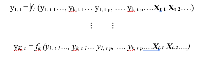
This kind of series allow us to model the dynamics of the series itself and also the interdependence of other series. We will explore this inter-dependence through Granger’s Causality Analysis.
Exploratory analysis:
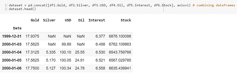
Let’s load the data and do some analysis with visualization to know insights of the data. Exploratory data analysis is quite extensive in multivariate time series. I will cover some areas here to get insights of the data. However, it is advisable to conduct all statistical tests to ensure our clear understanding on data distribution.
Let’s fix the dates for all the series.
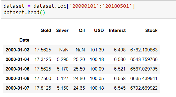
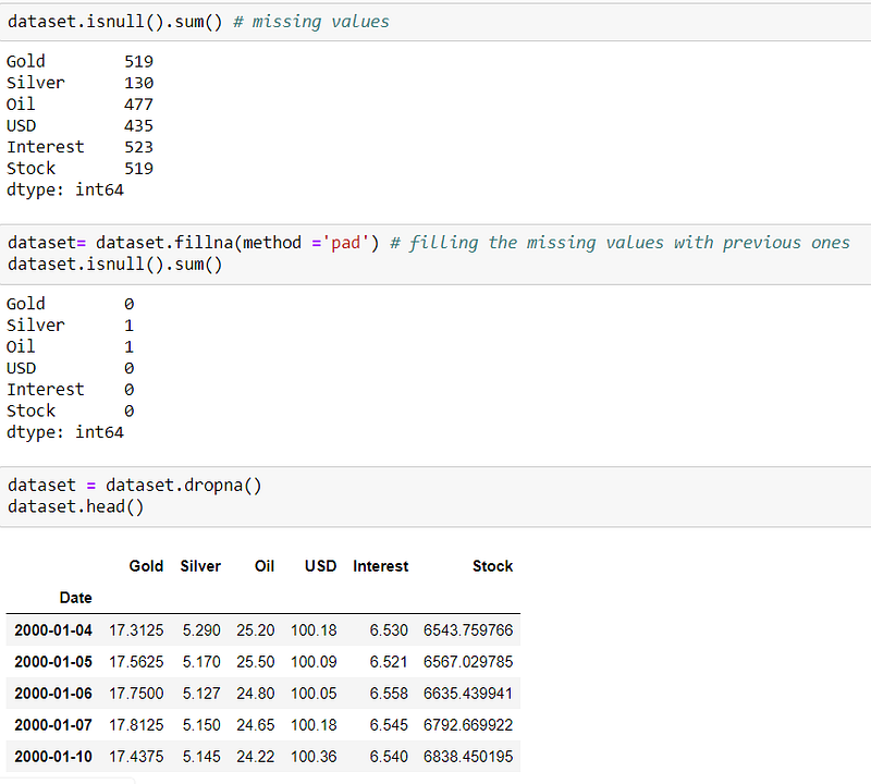
The NaN values in the data are filled with previous days data. After doing some necessary pre-processing, the dataset now clean for further analysis.
# Plot
fig, axes = plt.subplots(nrows=3, ncols=2, dpi=120, figsize=(10,6))
for i, ax in enumerate(axes.flatten()):
 data = dataset[dataset.columns[i]]
 ax.plot(data, color=’red’, linewidth=1)
 ax.set_title(dataset.columns[i])
 ax.xaxis.set_ticks_position(‘none’)
 ax.yaxis.set_ticks_position(‘none’)
 ax.spines[“top”].set_alpha(0)
ax.tick_params(labelsize=6)plt.tight_layout();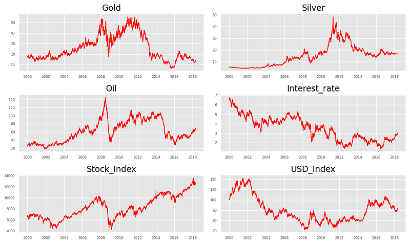
From the above plots, we can visible conclude that, all the series contain unit root with stochastic trend showing a systematic pattern that is unpredictable.
To extract maximum information from our data, it is important to have a normal or Gaussian distribution of the data. To check for that, we have done a normality test based on the Null and Alternate Hypothesis intuition.
stat,p = stats.normaltest(dataset.Gold)
print("Statistics = %.3f, p=%.3f" % (stat,p))
alpha = 0.05
if p> alpha:
print('Data looks Gaussian (fail to reject null hypothesis)')
else:
print('Data looks non-Gaussian (reject null hypothesis')output: Statistics = 658.293, p=0.000 Data looks Gaussian (reject null hypothesis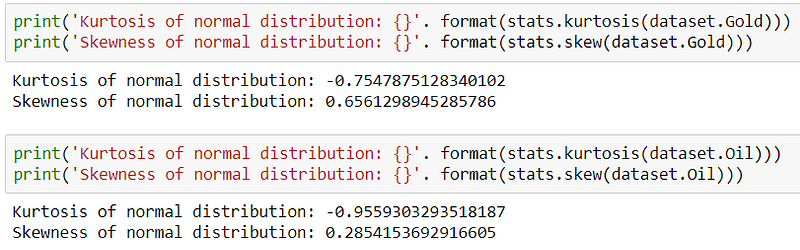
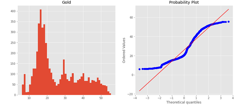
These two distributions give us some intuition about the distribution of our data. The kurtosis of this dataset is -0.95. Since this value is less than 0, it is considered to be a light-tailed dataset. It has as much data in each tail as it does in the peak. Moderate skewness refers to the value between -1 and -0.5 or 0.5 and 1.
plt.figure(figsize=(14,6))
plt.subplot(1,2,1)
dataset['Gold'].hist(bins=50)
plt.title('Gold')
plt.subplot(1,2,2)
stats.probplot(dataset['Gold'], plot=plt);
dataset.Gold.describe().T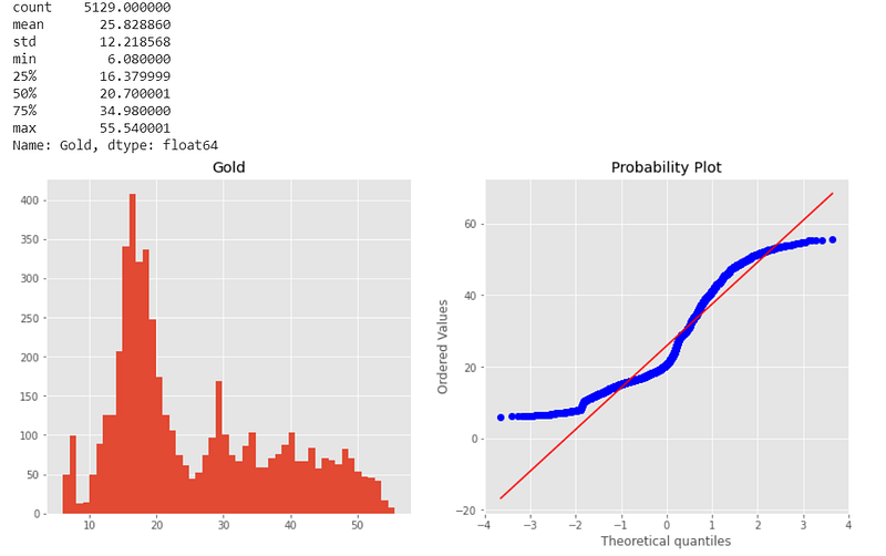
Normal probability plot also shows the data is far from normally distributed.
Auto-correlation:
Auto-correlation or serial correlation can be a significant problem in analyzing historical data if we do not know how to look out for it.
# plots the autocorrelation plots for each stock's price at 50 lags
for i in dataset:
  plt_acf(dataset[i], lags = 50)
  plt.title('ACF for %s' % i)
  plt.show()
We see here from the above plots, the auto-correlation of +1 which represents a perfect positive correlation which means, an increase seen in one time series leads to a proportionate increase in the other time series. We definitely need to apply transformation and neutralize this to make the series stationary. It measures linear relationships; even if the auto-correlation is minuscule, there may still be a nonlinear relationship between a time series and a lagged version of itself.
Train and Test Data:
The VAR model will be fitted on X_train and then used to forecast the next 15 observations. These forecasts will be compared against the actual present in test data.
n_obs=15
X_train, X_test = dataset[0:-n_obs], dataset[-n_obs:]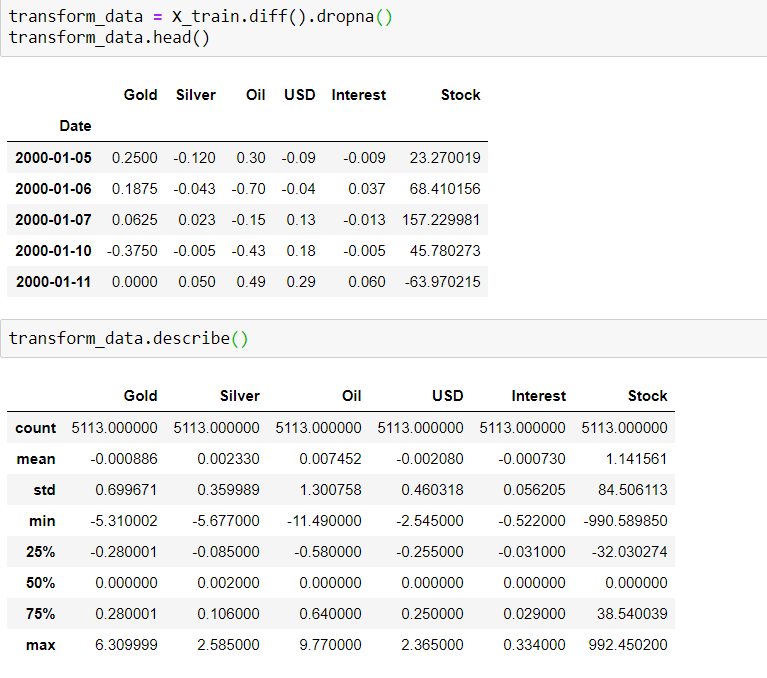
print(X_train.shape, X_test.shape)(5114, 6) (15, 6)Transformation:
Applying first differencing on training set to make all the series stationary. However, this is an iterative process where we after first differencing, the series may still be non-stationary. We shall have to apply second difference or log transformation to standardize the series in such cases.
Stationarity check:
def augmented_dickey_fuller_statistics(time_series):
  result = adfuller(time_series.values)
  print('ADF Statistic: %f' % result[0])
  print('p-value: %f' % result[1])
  print('Critical Values:')
  for key, value in result[4].items():
print('\t%s: %.3f' % (key, value))print('Augmented Dickey-Fuller Test: Gold Price Time Series')
augmented_dickey_fuller_statistics(X_train_transformed['Gold'])
print('Augmented Dickey-Fuller Test: Silver Price Time Series')
augmented_dickey_fuller_statistics(X_train_transformed['Silver'])
print('Augmented Dickey-Fuller Test: Oil Price Time Series')
augmented_dickey_fuller_statistics(X_train_transformed['Oil'])
print('Augmented Dickey-Fuller Test: Interest_rate Time Series')
augmented_dickey_fuller_statistics(X_train_transformed['Interest_rate'])
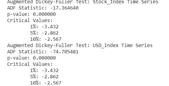
print('Augmented Dickey-Fuller Test: Stock_Index Time Series')
augmented_dickey_fuller_statistics(X_train_transformed['Stock_Index'])
print('Augmented Dickey-Fuller Test: USD_Index Time Series')
augmented_dickey_fuller_statistics(X_train_transformed['USD_Index'])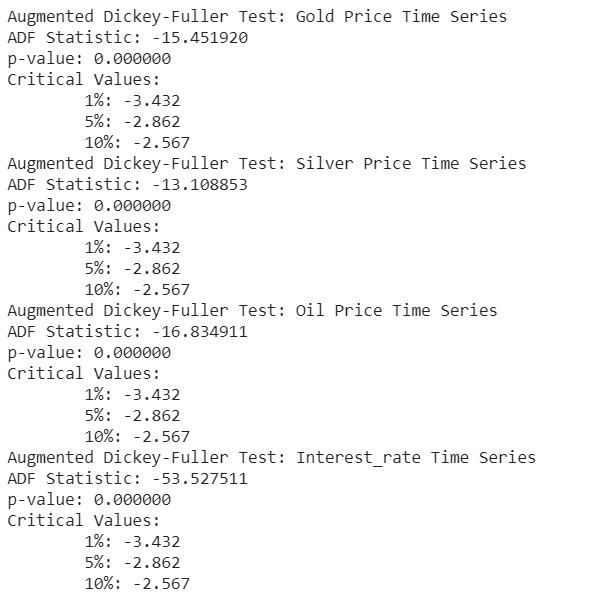
fig, axes = plt.subplots(nrows=3, ncols=2, dpi=120, figsize=(10,6))
for i, ax in enumerate(axes.flatten()):
d = X_train_transformed[X_train_transformed.columns[i]]
ax.plot(d, color='red', linewidth=1)
# Decorations
ax.set_title(dataset.columns[i])
ax.xaxis.set_ticks_position('none')
ax.yaxis.set_ticks_position('none')
ax.spines['top'].set_alpha(0)
ax.tick_params(labelsize=6)
plt.tight_layout();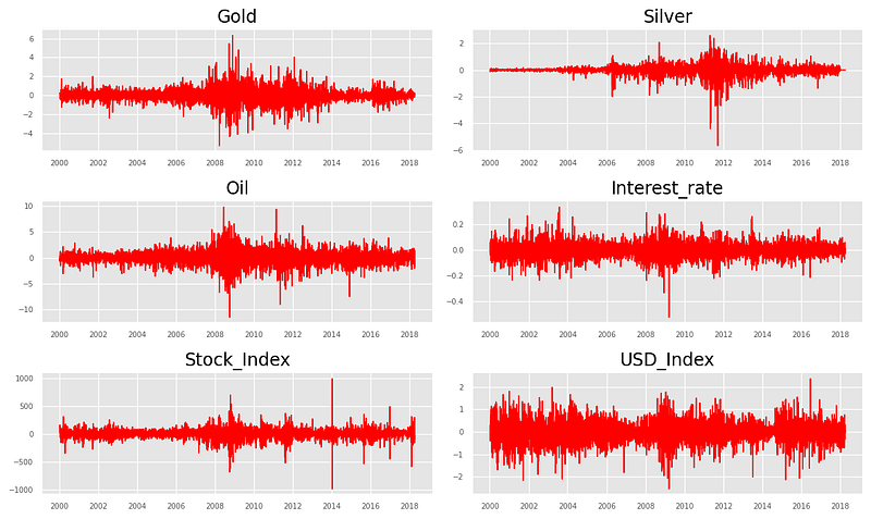
Granger’s Causality Test:
The formal definition of Granger causality can be explained as, whether past values of x aid in the prediction of yt, conditional on having already accounted for the effects on yt of past values of y (and perhaps of past values of other variables). If they do, the x is said to “Granger cause” y. So, the basis behind VAR is that each of the time series in the system influences each other.
Granger’s causality Tests the null hypothesis that the coefficients of past values in the regression equation is zero. So, if the p-value obtained from the test is lesser than the significance level of 0.05, then, you can safely reject the null hypothesis. This has been performed on original data-set.
Below piece of code taken from stackoverflow.
maxlag=12
test = 'ssr-chi2test'
def grangers_causality_matrix(X_train, variables, test = 'ssr_chi2test', verbose=False):
dataset = pd.DataFrame(np.zeros((len(variables), len(variables))), columns=variables, index=variables)
for c in dataset.columns:
for r in dataset.index:
test_result = grangercausalitytests(X_train[[r,c]], maxlag=maxlag, verbose=False)
p_values = [round(test_result[i+1][0][test][1],4) for i in range(maxlag)]
if verbose: print(f'Y = {r}, X = {c}, P Values = {p_values}')
min_p_value = np.min(p_values)
dataset.loc[r,c] = min_p_value
dataset.columns = [var + '_x' for var in variables]
dataset.index = [var + '_y' for var in variables]
return dataset
grangers_causality_matrix(dataset, variables = dataset.columns)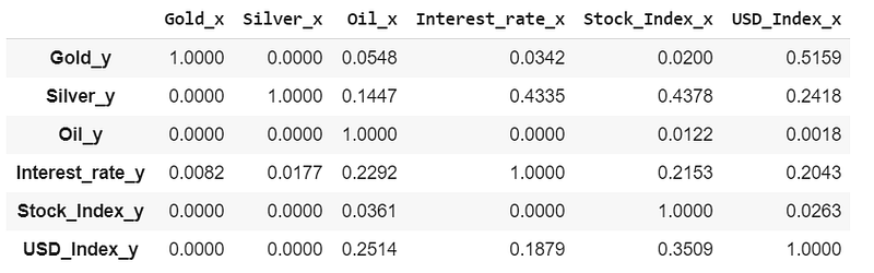
The row are the response (y) and the columns are the predictor series (x).
- If we take the value 0.0000 in (row 1, column 2), it refers to the p-value of the Granger’s Causality test for Silver_x causing Gold_y. The 0.0000 in (row 2, column 1) refers to the p-value of Gold_y causing Silver_x and so on.
- We can see that, in the case of Interest and USD variables, we cannot reject null hypothesis e.g. USD & Silver, USD & Oil. Our variables of interest are Gold and Oil here. So, for Gold, all the variables cause but for USD doesn’t causes any effect on Oil.
So, looking at the p-Values, we can assume that, except USD, all the other variables (time series) in the system are interchangeably causing each other. This justifies the VAR modeling approach for this system of multi time-series to forecast.
VAR model:
VAR requires stationarity of the series which means the mean to the series do not change over time (we can find this out from the plot drawn next to Augmented Dickey-Fuller Test).
Let’s understand the mathematical intuition of VAR model.
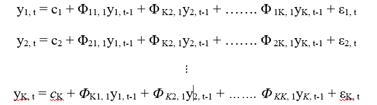
Here each series is modeled by it’s own lag and other series' lag. y{1,t-1, y{2,t-1}…. are the lag of time series y1,y2,…. respectively. The above equations are referred to as a VAR (1) model, because, each equation is of order 1, that is, it contains up to one lag of each of the predictors (y1, y2, …..). Since the y terms in the equations are interrelated, the y’s are considered as endogenous variables, rather than as exogenous predictors. To thwart the issue of structural instability, the VAR framework was utilized choosing the lag length according to AIC.
So, I will fit the VAR model on training set and then used the fitted model to forecast the next 15 observations. These forecasts will be compared against the actual present in test data. I have taken the maximum lag (15) to identify the required lags for VAR model.
mod = smt.VAR(X_train_transformed)
res = mod.fit(maxlags=15, ic='aic')
print(res.summary())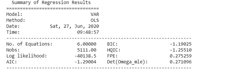
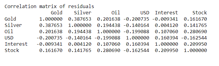
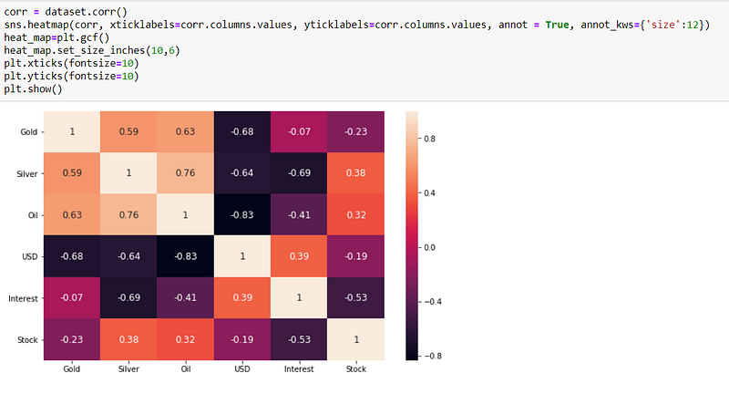
The biggest correlations are 0.38 (Silver & Gold) and -0.19 (Oil & USD); however, there are small enough to ignore in this case.
Residual plot:
Residual plot looks normal with constant mean throughout apart from some large fluctuation during 2009, 2011, 2014 etc.
y_fitted = res.fittedvalues
plt.figure(figsize = (15,5))
plt.plot(residuals, label='resid')
plt.plot(y_fitted, label='VAR prediction')
plt.xlabel('Date')
plt.xticks(rotation=45)
plt.ylabel('Residuals')
plt.grid(True)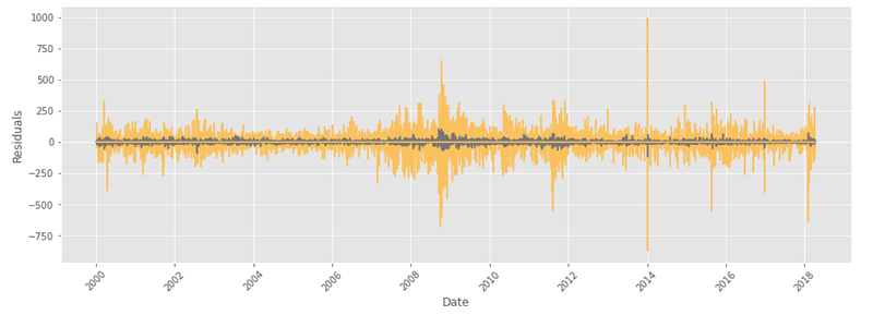
Durbin-Watson Statistic:
Durbin-Watson Statistic is related to related to auto correlation.
The Durbin-Watson statistic will always have a value between 0 and 4. A value of 2.0 means that there is no auto-correlation detected in the sample. Values from 0 to less than 2 indicate positive auto-correlation and values from 2 to 4 indicate negative auto-correlation. A rule of thumb is that test statistic values in the range of 1.5 to 2.5 are relatively normal. Any value outside this range could be a cause for concern.
A stock price displaying positive auto-correlation would indicate that the price yesterday has a positive correlation on the price today — so if the stock fell yesterday, it is also likely that it falls today. A stock that has a negative auto-correlation, on the other hand, has a negative influence on itself over time — so that if it fell yesterday, there is a greater likelihood it will rise today.
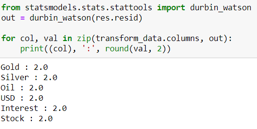
There is no auto-correlation (2.0) exist; so, we can proceed with the forecast.
Prediction:
In order to forecast, the VAR model expects up to the lag order number of observations from the past data. This is because, the terms in the VAR model are essentially the lags of the various time series in the data-set, so we need to provide as many of the previous values as indicated by the lag order used by the model.
# Get the lag order
lag_order = res.k_ar
print(lag_order)
# Input data for forecasting
input_data = X_train_transformed.values[-lag_order:]
print(input_data)# forecasting
pred = res.forecast(y=input_data, steps=n_obs)
pred = (pd.DataFrame(pred, index=X_test.index, columns=X_test.columns + '_pred'))
print(pred)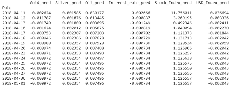
Invert the transformation:
The forecasts are generated but it is on the scale of the training data used by the model. So, to bring it back up to its original scale, we need to de-difference it.
The way to convert the differencing is to add these differences consecutively to the base number. An easy way to do it is to first determine the cumulative sum at index and then add it to the base number.
This process can be reversed by adding the observation at the prior time step to the difference value. inverted(ts) = differenced(ts) + observation(ts-1)
# inverting transformation
def invert_transformation(X_train, pred):
forecast = pred.copy()
columns = X_train.columns
for col in columns:
forecast[str(col)+'_pred'] = X_train[col].iloc[-1] + forecast[str(col)+'_pred'].cumsum()
return forecast
output = invert_transformation(X_train, pred)
#combining predicted and real data set
combine = pd.concat([output['Gold_pred'], X_test['Gold']], axis=1)
combine['accuracy'] = round(combine.apply(lambda row: row.Gold_pred /row.Gold *100, axis = 1),2)
combine['accuracy'] = pd.Series(["{0:.2f}%".format(val) for val in combine['accuracy']],index = combine.index)
combine = combine.round(decimals=2)
combine = combine.reset_index()
combine = combine.sort_values(by='Date', ascending=False)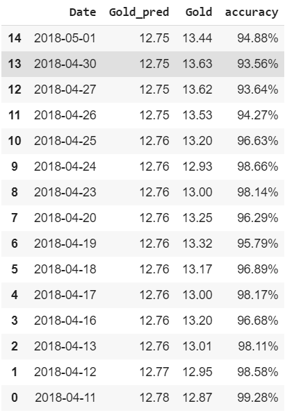
Evaluation:
To evaluate the forecasts, a comprehensive set of metrics, such as the MAPE, ME, MAE, MPE and RMSE can be computed. We have computed some of these as below.
#Forecast bias
forecast_errors = [combine['Gold'][i]- combine['Gold_pred'][i] for i in range(len(combine['Gold']))]
bias = sum(forecast_errors) * 1.0/len(combine['Gold'])
print('Bias: %f' % bias)print('Mean absolute error:', mean_absolute_error(combine['Gold'].values, combine['Gold_pred'].values))print('Mean squared error:', mean_squared_error(combine['Gold'].values, combine['Gold_pred'].values))print('Root mean squared error:', sqrt(mean_squared_error(combine['Gold'].values, combine['Gold_pred'].values)))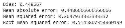
Mean absolute error tells us how big of an error we can expect from the forecast on average. Our error rates are quite low here indicating we have the right fit of the model.
Summary:
The VAR model is a popular tool for the purpose of predicting joint dynamics of multiple time series based on linear functions of past observations. More analysis e.g. impulse response (IRF) and forecast error variance decomposition (FEVD) can also be done along-with VAR to for assessing the impacts of shock from one asset on another to assess the impacts of shock from one asset on another. However, I will keep this simple here for easy understanding. In real-life business case, we should do multiple models with different approach to do the comparative analysis before zeroed down on one or a hybrid model.
I can be connected here.
Notice: The programs described here are experimental and should be used with caution. All such use at your own risk.


