Summary

This article explores the use of gradient boosting to enhance the performance of ARIMA models in time series forecasting, proposing a dynamic approach to parameter optimization for each round of boosting.

Abstract

The article delves into the application of gradient boosting to ARIMA models, a concept that has not been widely adopted in time series analysis despite its prevalence in machine learning. The author introduces ThymeBoost, a package developed to implement this approach, and demonstrates its capabilities using the Airline Passenger Dataset. The experiments reveal that static 'optimal' ARIMA parameters lead to poor performance when used in a boosting context. However, by allowing the model to search for new parameters at each boosting round, marginal improvements in forecasting accuracy can be achieved. Furthermore, the article suggests that combining ARIMA with other models, such as a linear trend, within the boosting framework can yield significant improvements over traditional methods. The findings advocate for a more dynamic and inclusive methodology in time series forecasting, highlighting the potential of leveraging multiple models in conjunction with gradient boosting.

Opinions

The author believes that traditional ARIMA models can be enhanced by incorporating gradient boosting techniques, despite the method's limited adoption in time series forecasting.
There is a skepticism towards using complex data partitioning methods in time series due to data limitations, which often lead to inferior results.
The article suggests that regularization of coefficients through boosting simple models, like linear regression, is less direct and potentially less effective than other regularization methods.
The author emphasizes that ThymeBoost's trend and seasonality assumptions are quite specific, which can affect the direct comparison with auto-ARIMA models.
The author expresses surprise and disappointment at the initial poor performance of boosted ARIMA models with static parameters, indicating a need for dynamic parameter optimization.
The author is optimistic about the potential of combining ARIMA with other forecasting methods, as demonstrated by the improved results when adding a linear trend to the boosting process.
The article concludes with encouragement for further exploration of boosting with time series methods, hinting at the success of ThymeBoost in the M4 Competition.

Gradient Boosted ARIMA for Time Series Forecasting

Boosting PmdArima’s Auto-Arima performance

TLDR: Adding gradient boosting to ARIMA adds complexity to the fitting procedure but can also drive accuracy if we optimize for new (p,d,q) parameters at each boosting round. Although, more gains can be achieved by boosting in conjunction with other methods.

All code lives here: ThymeBoost Github

For a full introduction to ThymeBoost view this article.

Introduction

Gradient Boosting has been a hot topic in the machine learning world for many years, but has yet to pick up much steam in the time series world. There has been theoretical work done, but not much has achieved mainstream attention like traditional methods such as ARIMA. This is primarily due to most of the gains from a boosting approach (typically) coming from methods which partition your data in some way such as decision trees. We could of course try to partition our data in some way, but many times we don’t have enough data to use very complex methods which leads to inferior results. On the other hand, boosting something simple such as a linear regression tends to regularize the coefficients but more direct methods of regularization are typically done.

With that said, let’s boost some time series methods!

Specifically, we will be looking at boosting ARIMA and comparing it against PmdArima. To do the boosting we will be using a package I am developing: ThymeBoost. This package uses a general boosting framework to do time series decomposition and forecasting, all the while embracing some of the more useful ideas found in gradient boosting that aren’t typically applied (from what I have seen). But for our purposes, we will just be doing simple boosting.

Our experiment will use a pretty common time series dataset to:

Fit an auto-arima from PmdArima
Use the parameters found to boost a simple ARIMA
Boost with PmdArima to search for new parameters at each round
Compare the results!

Airline Passenger Dataset

The first dataset we will try out is the Airline Passenger Dataset which can be found from Kaggle and comes with an Open Database license . Let’s take a look and import all the necessary packages:

import numpy as np
import pandas as pd
from matplotlib import pyplot as plt
import seaborn as sns
sns.set_style("darkgrid")#Airlines Data, if your csv is in a different filepath adjust this
df = pd.read_csv('AirPassengers.csv')
df.index = pd.to_datetime(df['Month'])
y = df['#Passengers']
plt.plot(y)
plt.show()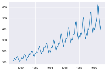

In order to judge the forecasting methods, we will split the data into a standard train/test split where the last 30% of the data is held out.

test_len = int(len(y) * 0.3)
al_train, al_test = y.iloc[:-test_len], y.iloc[-test_len:]

Now for a quick caveat, ThymeBoost makes some pretty specific assumptions on trend and seasonality so we can’t directly compare it with auto-arima while using seasonality (which this time series clearly has). But, we will try it anyway just with no seasonality.

First we use PmdArima:

import pmdarima as pm
# Fit a simple auto_arima model
arima = pm.auto_arima(al_train,
                      seasonal=False,
                      trace=True,
                      )
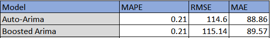
pmd_predictions = arima.predict(n_periods=len(al_test))
arima_mae = np.mean(np.abs(al_test - pmd_predictions))
arima_rmse = (np.mean((al_test - pmd_predictions)**2))**.5
arima_mape = np.sum(np.abs(pmd_predictions - al_test)) / (np.sum((np.abs(al_test))))

and the results:

Now, we will take the ‘optimal’ parameters and pass this to ThymeBoost to use for each boosting round. The order used is just the order in the PmdArima dict and the trend parameter (if I understand the documentation) will be ‘c’ when using an intercept. These parameters will be passed along to ThymeBoost:

#get the order
auto_order = arima.get_params()['order']
from ThymeBoost import ThymeBoost as tb
boosted_model = tb.ThymeBoost(verbose=1)

output = boosted_model.fit(al_train,
                            trend_estimator='arima',
                            arima_order=auto_order,
                            global_cost='mse')
predicted_output = boosted_model.predict(output, len(al_test))
tb_mae = np.mean(np.abs(al_test - predicted_output['predictions']))
tb_rmse = (np.mean((al_test - predicted_output['predictions'])**2))**.5
tb_mape = np.sum(np.abs(predicted_output['predictions'] - al_test)) / (np.sum((np.abs(al_test))))

and the results….are quite bad:

When looking at the predictions it is easy to see why:

boosted_model.plot_results(output, predicted_output)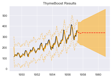

It appears the initialization round that occurs when boosting (fitting a simple mean/median) renders the previously found parameters useless. In fact, if you look at the logs, no boosting even occurs! The boosting procedure in ThymeBoost completely changes the game, negatively.

But, what if try to search for new parameters using PmdArima?

Let’s try it out.

To do this with ThymeBoost, we simply need to pass ‘auto’ for the arima_order parameter. Let’s see how it does:

from ThymeBoost import ThymeBoost as tb
boosted_model = tb.ThymeBoost(verbose=1)

output = boosted_model.fit(al_train,
                            trend_estimator='arima',
                            arima_order='auto',
                            global_cost='mse')
predicted_output = boosted_model.predict(output, len(al_test))
tb_mae = np.mean(np.abs(al_test - predicted_output['predictions']))
tb_rmse = (np.mean((al_test - predicted_output['predictions'])**2))**.5
tb_mape = np.sum(np.abs(predicted_output['predictions'] - al_test)) / (np.sum((np.abs(al_test))))

and the results:

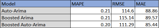
A slight improvement! Reviewing the logs we see 4 total rounds: 1 initialization round and 3 rounds of boosting.

But, we aren’t here for marginal improvements. Let’s boost with a simple linear trend in addition to an Auto-Arima to see how it does. This can be done by simply passing them as a list:

from ThymeBoost import ThymeBoost as tb
boosted_model = tb.ThymeBoost(verbose=1)

output = boosted_model.fit(al_train,
                            trend_estimator=['linear', 'arima'],
                            arima_order='auto',
                            global_cost='mse')
predicted_output = boosted_model.predict(output, len(al_test))
tb_mae = np.mean(np.abs(al_test - predicted_output['predictions']))
tb_rmse = (np.mean((al_test - predicted_output['predictions'])**2))**.5
tb_mape = np.sum(np.abs(predicted_output['predictions'] - al_test)) / (np.sum((np.abs(al_test))))

and the results:

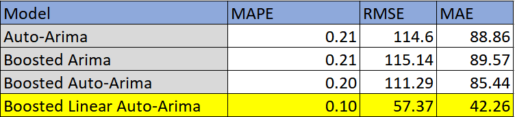
A significant improvement over all of the other methods!

Conclusion

In this article, we explored a boosting methodology utilizing ARIMA. We saw that taking a static ‘optimal’ parameter configuration can lead to horrifying results in the boosting procedure. On the other hand, if we dynamically find new parameter settings for each boosting round, we can make marginal gains in accuracy.

But, maybe just boosting an ARIMA is not always the best thing. Instead, maybe boosting ARIMAs with other models may lead us to better performance.

If you enjoyed this look at boosting with time series methods I highly recommend you check out my other article: The M4 Competition with ThymeBoost. This article is a first in a series where we will apply many wonky different ThymeBoost settings in an effort to learn how all of these methods work in the framework and to ultimately (spoiler warning) win the M4 Competition.