
Going Deep: An Introduction to Depth Estimation with Fully Convolutional Residual Networks
Have you ever looked at a two-dimensional image and wished you could know the depth of the objects in the scene? Perhaps you’re a computer vision researcher trying to build an autonomous vehicle that can accurately gauge distances, or a filmmaker seeking to create a more immersive virtual reality experience. Whatever your motivations may be, depth estimation is a fascinating and challenging task that has applications in a wide range of fields.
In this blog post, we’ll explore the task of depth estimation and its use cases. We’ll then dive into the details of how fully convolutional residual networks work, and show how they can achieve state-of-the-art results in depth estimation. Whether you’re a seasoned computer vision expert or just getting started in the field, you’re sure to learn something new about this exciting area of research.
Introduction & use cases
Depth estimation involves determining the distances between objects in a scene and the viewer’s point of view. Traditionally, this has been done with specialized hardware such as stereo cameras or depth sensors, but recent advancements in deep learning have led to the development of fully convolutional residual networks (FCRN) that can estimate depth from 2D images alone. This approach has significant potential to open up new possibilities for applications in robotics, virtual reality, and other domains.
Use cases
- Autonomous driving: Depth estimation can help self-driving cars determine the distances between objects in the environment, allowing them to make more informed decisions about steering, braking, and acceleration.
- Virtual and augmented reality: Depth estimation can enhance the realism of virtual and augmented reality experiences by allowing the system to accurately place virtual objects in the 3D space of the real world.
- Robotics: Depth estimation can help robots navigate and interact with their environments more effectively, whether in a factory setting or a household environment.
- Medical imaging: Depth estimation can help medical professionals create more accurate 3D models of the human body, which can be used for diagnosis, surgical planning, and research.
- Agriculture: Depth estimation can be used to measure the distances of crops, which can help farmers estimate yields and optimize irrigation and fertilizer usage.
Deeper Depth Prediction’s approach
This approach tackles the issue of depth estimation from a 2D image by using fully convolutional neural networks. The proposed model includes convolutional and transpose-convolutional layers, as well as residual up-sampling blocks that enable the network to address the challenging task of inferring depth from a single RGB image.
The research paper exposing the model explains how the network leverages residual learning in order to obtain an accurate depth map from the RGB image. The model is optimized using the Huber loss function and is capable of running at a steady frame rate of 30 FPS on images and videos.
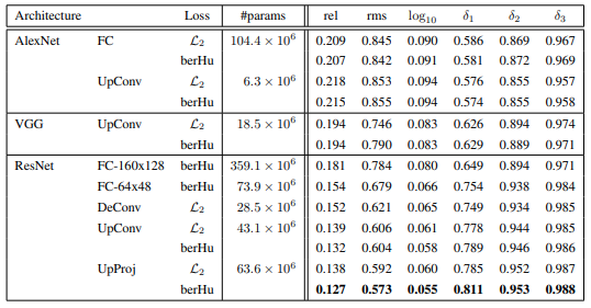
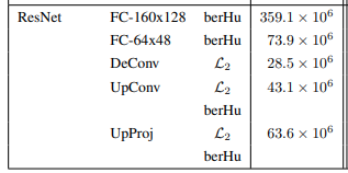
The FCRN architecture is a model mostly used for on-device depth prediction, which combines a fully convolutional model with up-sampling blocks. Various CNN variants of the FCRN architecture were tested, and it was found that fully connected networks on AlexNet were outperformed by fully convolutional ones, and VGG-based models with fully connected layers showed better results due to their multi-scale architecture. ResNet with fully connected layers showed similar performance to VGG-based models but with fewer data. The proposed architecture, ResNet-UpProj, with up-projection blocks, yielded the best results of all
Going deeper: Fully Convolutional Residual Networks
ResNet-50 is the foundation of the FCRN model, very popular for on-device depth prediction. This model was made famous when Apple utilized it in the depth sensors of their iPhone range, because compression and quantization for mobile deployment were relatively easy.
In this article, we’ll look at the important components and building blocks of the FCRN architecture, as well as its implementation in Pytorch.
Implementation
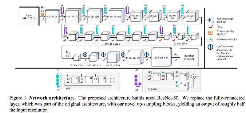
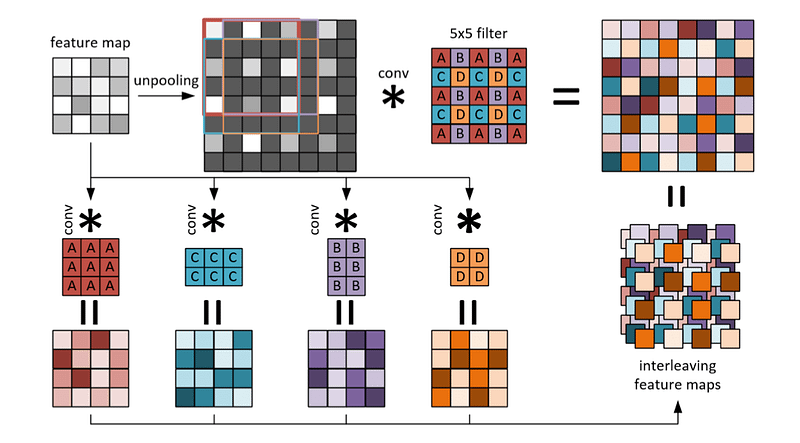
The FCRN architecture combines a fully convolutional model with novel up-sampling blocks (the ResNet-50 + UpProj), allowing for dense output maps of higher resolution while using fewer parameters and training on one order of magnitude fewer data than the state-of-the-art (at the time). The second part of the architecture guides the network into learning its upscaling through a sequence of unpooling and convolutional layers. Following the set of these upsampling blocks, dropout is applied and succeeded by a final convolutional layer yielding the prediction. I highly advice to read more about Up-Projection in the official paper:
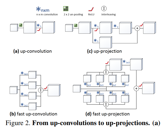
It also uses an efficient up-convolution scheme and combines it with the concept of residual learning to create up-projection blocks (efficient residual up-sampling blocks) for effective feature map upsampling.
The network is then trained by optimizing a reverse Huber loss (berHu) function.
Let’s start by defining the most important blocks of the architecture, the faster up-projection blocks:
class FasterUpConv(nn.Module):

    def __init__(self, in_channels):
        super(FasterUpConv, self).__init__()

        self.conv1_ = nn.Sequential(OrderedDict([
            ('conv1', nn.Conv2d(in_channels, in_channels // 2, kernel_size=3)),
            ('bn1', nn.BatchNorm2d(in_channels // 2)),
        ]))

        self.conv2_ = nn.Sequential(OrderedDict([
            ('conv1', nn.Conv2d(in_channels, in_channels // 2, kernel_size=(2, 3))),
            ('bn1', nn.BatchNorm2d(in_channels // 2)),
        ]))

        self.conv3_ = nn.Sequential(OrderedDict([
            ('conv1', nn.Conv2d(in_channels, in_channels // 2, kernel_size=(3, 2))),
            ('bn1', nn.BatchNorm2d(in_channels // 2)),
        ]))

        self.conv4_ = nn.Sequential(OrderedDict([
            ('conv1', nn.Conv2d(in_channels, in_channels // 2, kernel_size=2)),
            ('bn1', nn.BatchNorm2d(in_channels // 2)),
        ]))

        self.ps = nn.PixelShuffle(2)
        self.relu = nn.ReLU(inplace=True)

    def forward(self, x):
        x1 = self.conv1_(nn.functional.pad(x, (1, 1, 1, 1)))
        x2 = self.conv2_(nn.functional.pad(x, (1, 1, 0, 1)))
        x3 = self.conv3_(nn.functional.pad(x, (0, 1, 1, 1)))
        x4 = self.conv4_(nn.functional.pad(x, (0, 1, 0, 1)))

        x = torch.cat((x1, x2, x3, x4), dim=1)

        x = self.ps(x)
        return x
The given code defines a PyTorch module named FasterUpConv which performs upsampling on 2D images. The module contains four convolutional layers (self.conv1_, self.conv2_, self.conv3_, and self.conv4_) that have different kernel sizes to learn to upscale the input image in different directions. Each convolutional layer is followed by a batch normalization layer (nn.BatchNorm2d) to stabilize the training.
The module also contains a nn.PixelShuffle layer that reorganizes the elements of a tensor by merging groups of neighboring elements and reshaping them to form larger elements. The nn.ReLU layer applies the ReLU activation function to the output of the module.
The forward method of the module takes an input tensor (x) as its argument and performs padding on the input tensor using nn.functional.pad to ensure that the size of the output tensor matches the desired size. The padded tensor is then passed through each of the convolutional layers and the resulting tensors are concatenated along the channel dimension using torch.cat. Finally, the concatenated tensor is passed through the nn.PixelShuffle layer and the output is returned.
class FasterUpProjModule(nn.Module):
    def __init__(self, in_channels):
        super(FasterUpProjModule, self).__init__()
        out_channels = in_channels // 2

        self.upper_branch = nn.Sequential(collections.OrderedDict([
            ('faster_upconv', FasterUpConv(in_channels)),
            ('relu', nn.ReLU(inplace=True)),
            ('conv', nn.Conv2d(out_channels, out_channels,
             kernel_size=3, stride=1, padding=1, bias=False)),
            ('batchnorm', nn.BatchNorm2d(out_channels)),
        ]))
        self.bottom_branch = FasterUpConv(in_channels)
        self.relu = nn.ReLU(inplace=True)

    def forward(self, x):
        x1 = self.upper_branch(x)
        x2 = self.bottom_branch(x)
        x = x1 + x2
        x = self.relu(x)
        return x
The module takes an input tensor of in_channels and outputs a tensor of the same shape. The input tensor is first passed through two branches, the upper branch and the bottom branch, and the outputs are added together element-wise.
The upper branch starts with a FasterUpConv layer which upsamples the input tensor using four convolutional layers with different kernel sizes and then combines the outputs using pixel shuffling. The resulting tensor is then passed through a ReLU activation function, a 3x3 convolutional layer, and a batch normalization layer.
The bottom branch is another FasterUpConv layer that upsamples the input tensor using the same four convolutional layers as the upper branch.
Finally, the outputs of the two branches are added together element-wise, and the result is passed through another ReLU activation function before being returned as the output of the module. The purpose of this building block is to enable the network to learn how to upsample feature maps effectively by combining both learned and interpolated feature maps.
And finally:
class FasterUpProj(nn.Module):
    def __init__(self, in_channel):
        super(FasterUpProj, self).__init__()

        self.layer1 = FasterUpProjModule(in_channel)
        self.layer2 = FasterUpProjModule(in_channel // 2)
        self.layer3 = FasterUpProjModule(in_channel // 4)
        self.layer4 = FasterUpProjModule(in_channel // 8)

    def forward(self, x):
        x = self.layer1(x)
        x = self.layer2(x)
        x = self.layer3(x)
        x = self.layer4(x)
        return x
This implements the Faster Up-Projection module. The constructor takes an input channel parameter, and it initializes four FasterUpProjModule layers using the input channel parameter and its successive halving as the number of input channels.
The forward method takes an input tensor x and passes it through the four FasterUpProjModulelayers, one after the other, and returns the final output tensor. Each FasterUpProjModule layer consists of two parallel branches: an upper branch that applies a sequence of operations involving FasterUpConv, ReLU, Conv2d, and BatchNorm2d, and a bottom branch that applies only the FasterUpConv operation. The outputs of the two branches are added together element-wise.
Last but not least, let’s put everything together to define the Resnet50-UpProj:
class ResNet(nn.Module):
    def __init__(self, layers=50, output_size=(228, 304), in_channels=3, pretrained=True):
        super(ResNet, self).__init__()

        pretrained_model = torchvision.models.__dict__[f'resnet{layers}'](pretrained=pretrained)

        self.conv1 = pretrained_model.conv1
        self.bn1 = pretrained_model.bn1
        self.output_size = output_size
        self.relu = pretrained_model.relu
        self.maxpool = pretrained_model.maxpool
        self.layer1 = pretrained_model.layer1
        self.layer2 = pretrained_model.layer2
        self.layer3 = pretrained_model.layer3
        self.layer4 = pretrained_model.layer4

        del pretrained_model #free memory

        num_channels = 512 if layers <= 34 else 2048

        self.conv2 = nn.Conv2d(num_channels, num_channels // 2, kernel_size=1, bias=False)
        self.bn2 = nn.BatchNorm2d(num_channels // 2)
        self.upsample = FasterUpProj(num_channels // 2)
        self.conv3 = nn.Conv2d(num_channels // 32, 1, kernel_size=3, stride=1, padding=1, bias=False)
        self.bilinear = nn.Upsample(size=self.output_size, mode='bilinear', align_corners=True)

        self.conv2.apply(weights_init)
        self.bn2.apply(weights_init)
        self.upsample.apply(weights_init)
        self.conv3.apply(weights_init)

    def forward(self, x):
        x = self.conv1(x)
        x = self.bn1(x)
        x = self.relu(x)
        x = self.maxpool(x)
        x1 = self.layer1(x)
        x2 = self.layer2(x1)
        x3 = self.layer3(x2)
        x4 = self.layer4(x3)

        x = self.conv2(x4)
        x = self.bn2(x)
        x = self.upsample(x)
        x = self.conv3(x)
        x = self.bilinear(x)

        return x
The weights_init function is an utility one to initialize the weights and it’s defined as follows:
def weights_init(m):
    """
    Initializes the weights of the convolutional and batch normalization layers in a neural network.

    Args:
        m (nn.Module): A neural network module.

    Returns:
        None

    Notes:
        The function initializes the weights of the convolutional and batch normalization layers in a neural network
        with random values drawn from a normal distribution with a mean of zero and a variance of 2/n, where n is the
        number of input neurons to the layer. If the layer has a bias term, it is initialized to zero.
    """
    if isinstance(m, nn.Conv2d):
        n = m.kernel_size[0] * m.kernel_size[1] * m.out_channels
        m.weight.data.normal_(0, math.sqrt(2. / n))
        if m.bias is not None:
            m.bias.data.zero_()
    elif isinstance(m, nn.ConvTranspose2d):
        n = m.kernel_size[0] * m.kernel_size[1] * m.in_channels
        m.weight.data.normal_(0, math.sqrt(2. / n))
        if m.bias is not None:
            m.bias.data.zero_()
    elif isinstance(m, nn.BatchNorm2d):
        m.weight.data.fill_(1)
        m.bias.data.zero_()
Here’s the torchsummary’s report:
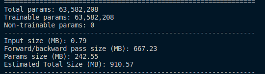
Around 63.6 millions of parameters, like in the proposed architecture from the paper:
Training on the NYUv2 dataset
I highly recommend to checkout the Pytorch implementation of the paper, especially for downloading and using the NYUv2 dataset. In the meantime, I’ll leave here some code to get you started!
The loss function As said above, the paper leverages an inverse Huber loss function to optimize the model, and can be defined as follows:
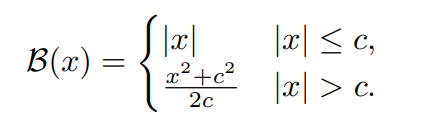
class berHuLoss(nn.Module):
    def __init__(self):
        super(berHuLoss, self).__init__()

    def forward(self, pred, target, delta=1.0):
        assert pred.dim() == target.dim(), "inconsistent dimensions"

        error = target - pred
        abs_error = torch.abs(error)
        mask = abs_error < delta
        squared_loss = 0.5 * torch.square(error)
        linear_loss = delta * (abs_error - 0.5 * delta)
        loss = torch.where(mask, squared_loss, linear_loss)
        return torch.mean(loss)
The rest is the good ol’ training loop which is plain boilerplate by now:
optimizer = torch.optim.SGD(net.parameters(), lr=0.01, momentum=0.9, weight_decay=0.0005)
criterion = berHuLoss()
scheduler = lr_scheduler.ReduceLROnPlateau(
optimizer, 'min', patience=5, verbose=True)
for epoch in range(1, 100):
net.train()
for i, (rgb, depth) in enumerate(train_loader):
rgb = rgb.cuda()
depth = depth.cuda()
output = net(rgb)
loss = criterion(output, depth)
optimizer.zero_grad()
loss.backward()
optimizer.step()
torch.cuda.synchronize()
rmse = torch.sqrt(torch.mean((output - depth) ** 2))
print("Epoch: {}, Iter: {}, Loss: {}, RMSE: {}".format(epoch, i, loss.item(), rmse.item()))
scheduler.step(loss)
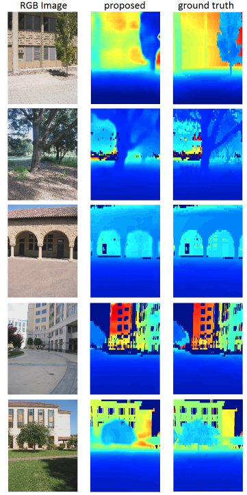
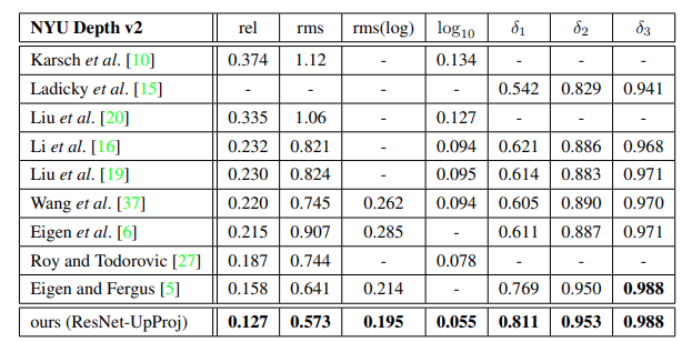
torch.save(net.state_dict(), "fcrn.pth")I’ll leave you play with the transformations to apply to the images! Here’s the results from the paper:
Conclusion
In conclusion, depth estimation is an important task in computer vision that has numerous applications in areas such as robotics, augmented reality, and autonomous driving. We discussed some of the use cases of depth estimation, including 3D reconstruction, object detection, and scene understanding.
We also implemented the Fully Convolutional Residual Network (FCRN), which is a popular method for monocular depth estimation. We used PyTorch to implement the FCRN architecture and trained it on the NYU Depth v2 dataset.
If you want to keep in touch with me:


