
Getting Started with Machine Learning (Part 2): An Absolute Beginner’s Guide — Plotting

Plotting the Top 11 machine learning algorithms
- Linear Regression: Linear regression is a supervised machine learning algorithm for predicting continuous values. It is one of the most widely used algorithms to model the relationship between a dependent variable and one or more independent variables. It is implemented in Python with the help of the scikit-learn library.
# sample code -> LinearRegression
# import libraries
import numpy as np
from sklearn.linear_model import LinearRegression
import matplotlib.pyplot as plt

# generate dummy linear data
x = np.arange(100)
y = 3 * x + 4 + np.random.randn(100)

# create a linear regression object
model = LinearRegression()

# train the model using the data
model.fit(x.reshape(-1, 1), y)

# make predictions using the trained model
y_pred = model.predict(x.reshape(- 1, 1))

# plot the data points and the fitted line
plt.scatter(x, y)
plt.plot(x, y_pred, color='red')

# format scatter plot
plt.title('Linear Regression')
plt.xlabel('x')
plt.ylabel('y')

# display plot
plt.show()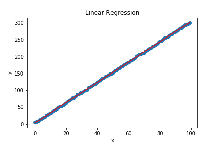
2. Logistic Regression: Logistic regression is an extension of linear regression used to predict binary values (Yes/No). It is used to model the probability of an event occurring. For example, it is often used to indicate an individual’s likelihood of belonging to a particular class or group. It is implemented in Python with the help of the scikit-learn library.
# sample code -> LogisticRegression
# import libraries
import numpy as np
from sklearn.linear_model import LogisticRegression
import matplotlib.pyplot as plt
from sklearn import tree

# generate dummy logistic data
x = np.random.randn(100, 2)
y = np.random.randint(0, 2, size=100)

# create a logistic regression object
model = LogisticRegression()

# train the model
model.fit(x.reshape(-1, 1), y)

# make predictions using the trained model
y_pred = model.predict(x.reshape(- 1, 1))

# plot the data points and the fitted line
plt.scatter(x, y)
plt.plot(x, y_pred, color='red')

# format scatter plot
plt.title('Logistic Regression')
plt.xlabel('x')
plt.ylabel('y')

# display plot
plt.show()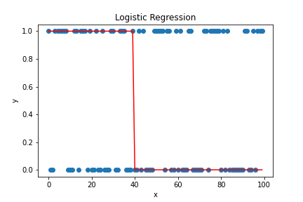
3. Support Vector Machine (SVM): SVM is a supervised machine learning algorithm for classification and regression problems. The goal is to find the best decision boundary that maximizes the distance between multiple classes’ closest data points (support vectors). It is implemented in Python with the help of the scikit-learn library.
# sample code -> Support Vector Classification
# import libraries
import numpy as np
from sklearn.svm import SVC
import matplotlib.pyplot as plt

# generate dummy svm data
x = np.random.randn(100, 2)
y = np.random.randint(2, size=100)

# create a svm object
model = SVC()

# train the model
model.fit(x, y)

# make predictions using the trained model
y_pred = model.predict(x)

# plot the data points and the fitted line
plt.scatter(x[:, 0], x[:, 1], c=y_pred)

# format scatter plot
plt.title('SVM')
plt.xlabel('x')
plt.ylabel('y')

# display plot
plt.show()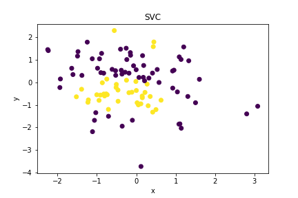
4. Decision Trees: Decision trees are a tree-like algorithm used to model decisions and their possible outcomes. It is used to solve classification and regression problems. It is implemented in Python with the help of the scikit-learn library.
# sample code -> DecisionTreeClassifier
# import libraries
import numpy as np
from sklearn.tree import DecisionTreeClassifier
import matplotlib.pyplot as plt
from sklearn import tree

# generate dummy decision tree data
# df = entire dataset
x = np.random.randn(100, 2)
y = np.random.randint(2, size=100)

# create a decision trees object
model = DecisionTreeClassifier(random_state=42)

# train the model
model.fit(x, y)

# extract text representation of model
text_representation = tree.export_text(model)

# create figure object
plt.figure(figsize=(25,20))

fig = tree.plot_tree(model,
                   # feature_names=df.feature_names,
                   # class_names=df.target_names,
                   filled=True)
# display plot
plt.show(fig)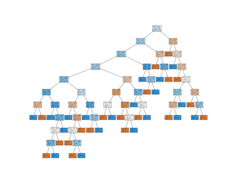
5. Hierarchical Clustering: Hierarchical clustering is the process of grouping data points into clusters based on similarity. It is used to analyze data and cluster it into meaningful groups. It is implemented in Python with the help of the scikit-learn library.
# sample code -> AgglomerativeClustering
# import libraries
import numpy as np
from sklearn.cluster import AgglomerativeClustering
import matplotlib.pyplot as plt

# generate dummy clustering data
x = np.random.randn(100, 2)
y = np.random.randint(2, size=100)

# create a agglomerative clustering object
model = AgglomerativeClustering(n_clusters=2)

# train the model
model.fit(x)

# make predictions using the trained model
y_pred = model.labels_

# plot the predicted clusters
plt.scatter(x[:, 0], x[:, 1], c=y_pred)

# format scatter plot
plt.title('Agglomerative Clustering')
plt.xlabel('x')
plt.ylabel('y')

# display plot
plt.show()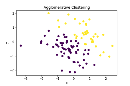
6. K-Means Clustering: K-Means clustering is an unsupervised learning algorithm that solves clustering problems. It is used to group data points into clusters based on their similarity. It is implemented in Python with the help of the scikit-learn library.
# sample code -> K-means
# import libraries
import numpy as np
from sklearn.cluster import KMeans
import matplotlib.pyplot as plt

# generate dummy clustering data
x = np.random.randn(100, 2)
y = np.random.randint(2, size=100)

# create a k-means clustering object
model = KMeans(n_clusters=2)

# train the model
model.fit(x)

# make predictions using the trained model
y_pred = model.predict(x)

# plot the predicted clusters
plt.scatter(x[:, 0], x[:, 1], c=y_pred)

# format scatter plot
plt.title('K-means Clustering')
plt.xlabel('x')
plt.ylabel('y')

# display plot
plt.show()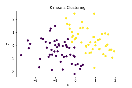
7. Naive Bayes: Naive Bayes is a supervised machine learning algorithm for classification and prediction. It is based on the Bayes theorem and calculates the probability of an event occurring given the evidence. It is implemented in Python with the help of the scikit-learn library
# sample code -> Linear Naive Bayes
# import libraries
import numpy as np
from sklearn.naive_bayes import GaussianNB
import numpy as np

# generate dummy data
x = np.random.randn(100, 2)
y = np.random.randint(2, size=100)

# create a gaussianNB object
model = GaussianNB()

# train the model
model.fit(x, y)

# make predictions using the trained model
y_pred = model.predict(x)

# plot the predicted labels
plt.scatter(x[:, 0], x[:, 1], c=y_pred)

# format the plot
plt.title('GaussianNB')
plt.xlabel('x')
plt.ylabel('y')

# display plot
plt.show()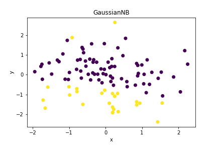
8. Random Forest: Random forest is an ensemble machine learning algorithm that solves classification and regression problems. It is based on decision trees and combines them to create an even more accurate and robust prediction model. It is implemented in Python with the help of the scikit-learn library.
# sample code -> Random Forest
# import libraries
import numpy as np
from sklearn.ensemble import RandomForestClassifier
import matplotlib.pyplot as plt

# generate dummy data
x = np.random.randn(100, 2)
y = np.random.randint(2, size=100)

# create a random forest object
model = RandomForestClassifier()

# train the model
model.fit(x, y)

# make predictions using the trained model
y_pred = model.predict(x)

# plot the predicted labels
plt.scatter(x[:, 0], x[:, 1], c=y_pred)

# format scatter plot
plt.title('Random Forest')
plt.xlabel('x')
plt.ylabel('y')

# display plot
plt.show()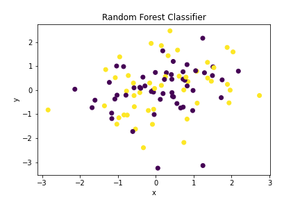
9. Gradient Boosting: Gradient boosting is an ensemble machine learning algorithm that solves regression and classification problems. It is based on decision trees and uses the residual errors of a model to build new models. It is implemented in Python with the help of the scikit-learn library.
# sample code -> GradientBoostingClassifier
# import libraries
import numpy as np
from sklearn.ensemble import GradientBoostingClassifier
import matplotlib.pyplot as plt

# generate dummy data
x = np.random.randn(100, 2)
y = np.random.randint(2, size=100)

# create a gradient boosting object
model = GradientBoostingClassifier()

# train the model
model.fit(x, y)

# make predictions using the trained model
y_pred = model.predict(x)

# plot the predicted labels
plt.scatter(x[:, 0], x[:, 1], c=y_pred)

# format the plot
plt.title('Gradient Boosting')
plt.xlabel('x')
plt.ylabel('y')

# display plot
plt.show()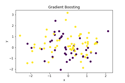
10. K-Nearest Neighbors (KNN): KNN is an unsupervised machine learning algorithm that solves classification and prediction problems. It is based on the similarity of a data point to its nearest neighbors and is used to predict the class of a data point. It is implemented in Python with the help of the scikit-learn library.
# sample code -> KNeighborsClassifier
# import libraries
import numpy as np
from sklearn.neighbors import KNeighborsClassifier
import matplotlib.pyplot as plt

# generate dummy data
x = np.random.randn(100, 2)
y = np.random.randint(2, size=100)

# create the model/neighbors object
model = KNeighborsClassifier(n_neighbors=3)

# train the model
model.fit(x, y)

# make predictions using the trained model
y_pred = model.predict(x)

# plot the predicted labels
plt.scatter(x[:, 0], x[:, 1], c=y_pred)

# format plot
plt.title('K-neighbors Classifier')
plt.xlabel('x')
plt.ylabel('y')

# display plot
plt.show()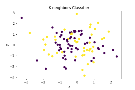
11. Dimensionality Reduction: Dimensionality reduction is an unsupervised machine learning algorithm used to reduce the number of features or dimensions of a dataset. It is used to make datasets easier to analyze and visualize. It is implemented in Python with the help of the scikit-learn library.
# sample code -> dimensionality reduction using principle component analysis
# import libraries
import numpy as np
from sklearn.preprocessing import StandardScaler
from sklearn.decomposition import PCA
import matplotlib.pyplot as plt


# generate dummy data
x = np.random.randn(100, 2)
y = np.random.randint(2, size=100)

# scale the data to be in a range of 0 - 1
scaler = StandardScaler()
x_scaled = scaler.fit_transform(x)

# create a PCA model
pca = PCA(n_components=2)

# train the model
pca.fit(x_scaled)

# make predictions using the trained model
y_pred = pca.transform(x_scaled)

# plot the predicted data
plt.scatter(y_pred[:, 0], y_pred[:, 1], c=y)

# format plot
plt.title('PCA')
plt.xlabel('x')
plt.ylabel('y')

# display plot
plt.show()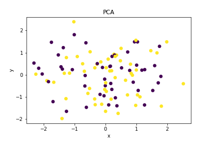
For additional PM and ML reading and resources (mixture of free and subscription services): Bits, Bytes, and Bots
For Education & Analytics reading and resources (mixture of free and subscription services): Education on Education


