
Get Uncertainty Estimates in Regression Neural Networks for Free
Given the right loss function, a standard neural network can output uncertainty as well

Whenever we build a machine learning model, we usually design it in such a way that it outputs a single number as the prediction. Most models from scikit-learn work like this: tree-based models, linear models, nearest neighbor algorithms, and more. The same goes for XGBoost and the other boosting algorithms, as well as for deep learning frameworks such as Tensorflow or PyTorch.
While this is often fine, it would be better to have a measure of uncertainty around this point estimate as well. This is because the difference between “We will sell 1000±50 cars” and “We will sell 1000±5000 cars” is tremendous: From the first statement, you can conclude that the company will sell around 1000 cars, give or take, while the second statement tells you that the model has no clue at all.
Note: A lower uncertainty does not mean that the model is right. As people, it can also be very opinionated about something completely wrong. So, as usual, assessing the model’s quality is essential, also in this case.
Bayesian Inference
If you have read my articles about Bayesian inference (thanks!) you already know how to create models that output not only a single point, but a complete target distribution instead.
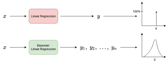
Because of this, we can see when the model is uncertain just by looking at the predicted distribution, or some derived number such as the standard deviation. The narrower the distribution (the smaller the standard deviation), the more certain the model is.
However, this time we will not go Bayesian here. While Bayesian inference is a great field that you should study at some point, it has several shortcomings:
- it is computationally even more involved than neural networks
- it is harder to understand mathematically, and
- you have to learn about new libraries.
So, this article is for the people that know their deep learning frameworks and want to include some uncertainty estimates without much hassle. However, if you feel like going into the realm of fully Bayesian neural networks at some point, try out libraries like Tensorflow Probability or Pyro for PyTorch.
Make Neural Networks Reveal Their Uncertainties
Disclaimer: Again, I do not know if the following method was presented in any paper or book. It just came to my mind and I wanted to write about it. If you know any source, please give me a hint in the comments and I will add it to the article. Thanks! Update: Matias Valdenegro Toro pointed out that the loss that I will introduce soon is called variance attenuation in their paper.
From now, let us stick with our favorite bread and butter neural networks. I will use Tensorflow code in this article but you can easily adapt everything to PyTorch or other frameworks as well. We will consider a regression problem here, but similar arguments can be made for classification tasks, too.
Deriving the Mean Squared Error
In order to understand how to get uncertainty estimates, we have to understand how to get point estimates first. We will then generalize this idea in a simple fashion. So, for a small recap, the following is the mean squared error (MSE) loss function:
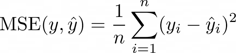
It makes sense intuitively: the larger the gap between some true value yᵢ and the model’s prediction ŷᵢ, the higher the loss. But we can argue in the same way when replacing the 2 with a 4 in the exponent. Or dropping the 2 and using the absolute value |yᵢ – ŷᵢ| instead (mean absolute error, MAE).
So, what is special about the MSE? Which assumptions go into it? Let us find out. ⚠️Danger: Math ahead. If this is too much, just skip to the implementation section. The results are easy to apply, even if you cannot follow the theory yet.⚠️
The assumption is the following:
Given input features x, the true label y is distributed according to a normal distribution with mean μ(x) and standard deviation σ, i.e. y~N(μ(x), σ²). This means that the observed labels come from some true value μ(x), but got corrupted by some error with a standard deviation of σ. This error is also called noise. Note that very often we write ŷ instead of μ(x).
The task of a neural network (and most other models) is then to predict this μ(x) given x. This makes predictions right on average, and this is the best thing we can do because we are not able to predict the noise. Now, the expression y~N(μ(x), σ²) just means the following:
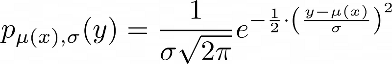
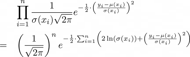
This is just the density function of the normal distribution with mean ŷ=μ(x) and standard deviation σ that describes the distribution of a single label y. Now, we don’t have a single observation y and its corresponding prediction ŷ, but several, let’s say n. Assuming that all observations are stochastically independent, we get

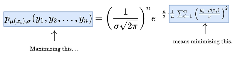
Training a neural network now basically means something that statisticians call maximum-likelihood estimation. This is a fancy way of saying that we want to maximize the above density function, also called the likelihood function.
Now, we can connect the maximum-likelihood estimation to the MSE minimization like this:
- Maximizing the likelihood function
- means maximizing the rightmost term
- means maximizing the exponent of e
- means minimizing the sum in the exponent,
- means minimizing the MSE (dividing by n does not change the optimal parameters).
Or as a picture:
Generalizing the MSE Loss
Congratulations if you survived the last section, you made it far, and you nearly reached your goal! We just have to make a simple observation:
We treated σ as a constant and basically ignored it when doing the maximum-likelihood approach.
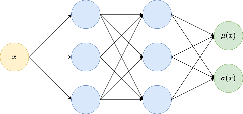
But σ is exactly what we want to estimate as well! This is because it captures the uncertainty in the predictions by definition. So, how about we let our model output a value σ(x) additionally to μ(x)? This means that even for a simple regression, the model will have two outputs: one estimate for the true value μ(x), and the uncertainty estimate σ(x) given x.
Now, we can just replace all the σ by σ(xᵢ) in the above equations and we end up with the following statement: Maximizing the likelihood function means maximizing the term
This in turn means minimizing the huge sum in the exponent, which is our newly derived loss function (without a catchy name, post suggestions in the comments 😉):
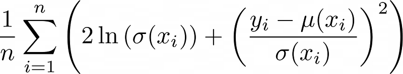
Note that I smuggled a 1/n in, but this does not change the optimal solution, as in the case of the MSE.
Note: This loss has some interesting properties. First, it still contains the MSE bit (yᵢ – μ(xᵢ))². Additionally, there are two terms involving σ: ln(σ(x)) as well as 1/σ(x).
In order to keep the loss low, the model cannot output very large values for σ(x) because as σ(x) grows, ln(σ(x)) increases as well. The model cannot output very small values close to zero either because then the term 1/σ(x) becomes large. Thus, the model is forced to output a reasonable guess for σ(x) to balance the penalty of both terms.
Only if (yᵢ — μ(xᵢ))² is small, i.e. the predicted value is quite close to the truth, the model can afford outputting a small standard deviation σ(x). In this case, the model is quite sure about its prediction.
Alright, enough of the theory. We deserved some coding now!
Implementation in Tensorflow
Alright, so we have learned that we need two things to make a standard neural network output uncertainty:
- A second output node that contains the predicted standard deviation (=uncertainty) and
- the custom loss function as stated above.
It should be easy to implement both things in any deep learning framework of your choice. We will do it in Tensorflow, just because last time I have already chosen PyTorch to explain interpretable neural networks. 😎
Let’s start with a simple example.
Constant Noise
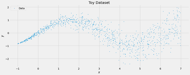
First, we will create a toy dataset consisting of 1000 points with constant noise via
import tensorflow as tf

tf.random.set_seed(0)

X = tf.random.uniform(minval=-1, maxval=7, shape=(1000,))
y = tf.sin(X) + tf.random.normal(mean=0, stddev=0.3, shape=(1000,))
We can visualize this dataset:
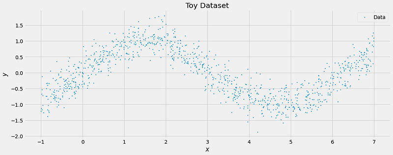
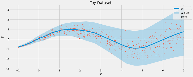
Alrighty, so it is merely a sine wave with N(0, 0.3²) distributed noise added to it. In the best case, the actual prediction of the model follows the sine wave, while each uncertainty estimate is around 0.3. We build a simple feed-forward network via
model = tf.keras.Sequential([
    tf.keras.layers.Dense(32, activation='relu'),
    tf.keras.layers.Dense(32, activation='relu'),
    tf.keras.layers.Dense(32, activation='relu'),
    tf.keras.layers.Dense(2) # Output = (μ, ln(σ))
])
Ok, so we dealt with the first ingredient already by defining a neural network with two outputs.
To simplify the computations, let us assume that the second output is not σ(xᵢ) directly, but ln(σ(xᵢ)) instead. We do this because the two neurons from the last layer can output arbitrary real values, especially values that are less than zero, which does not make sense for the standard deviation. But the logarithm of the standard deviation can be any real number, so the domains match then. And we need ln(σ(xᵢ)) in the loss function anyway, so let’s go for it. Speaking of the loss function, we can define it via
def loss(y_true, y_pred):
    mu = y_pred[:, :1] # first output neuron
    log_sig = y_pred[:, 1:] # second output neuron
    sig = tf.exp(log_sig) # undo the log

    return tf.reduce_mean(2*log_sig + ((y_true-mu)/sig)**2)
The rest is business as usual. You compile the model with this loss function and fit.
model.compile(loss=loss)

model.fit(
    tf.reshape(X, shape=(1000, 1)),
    tf.reshape(y, shape=(1000, 1)),
    batch_size=32,
    epochs=100
)
Let us check the uncertainty estimates that the model has learned:
print(tf.exp(model(X)[:20, 1]))

# Output:
# tf.Tensor(
# [0.29860803 0.27371496 0.32216415 0.32288837 0.31084406 0.30166912
# 0.32059005 0.3331769  0.31244662 0.31863096 0.30940703 0.32042852
# 0.3231969  0.29584357 0.31141806 0.32493973 0.3169802  0.32060665
# 0.30542135 0.31733593], shape=(20,), dtype=float32)
Looks good to me! The model learned that the noise has a standard deviation of around 0.3. And here is a visualization of what the model has learned:
That’s how we like it. The actual prediction μ follows the data while the uncertainty σ is just high enough to capture the noise in the labels y.
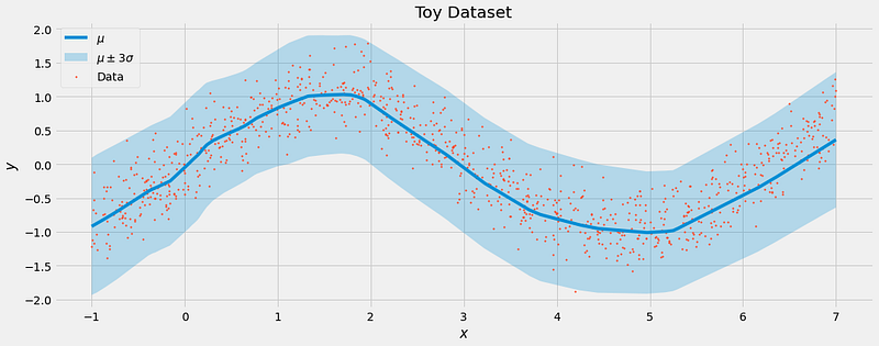
Varying Noise
We now spice things up a little bit by introducing non-constant noise, something that statisticians call heteroscedasticity. Take a look at this:
tf.random.set_seed(0)

X = tf.random.uniform(minval=-1, maxval=7, shape=(1000,))
sig = 0.1*(X+1)
y = tf.sin(X) + tf.random.normal(mean=0, stddev=sig, shape=(1000,))
This creates a dataset with noise increasing in feature X.
The ground truth is still the same: it’s a sine wave, and the model should be able to capture this. However, the model should also learn that higher values for X mean higher uncertainty.
Spoiler: If you re-train the same model as above on the new dataset, this is exactly what you will see.
Pretty sweet in my opinion.
Conclusion
In this article, you have learned how to tweak a neural network so that it can output estimates for uncertainty together with its actual prediction. All it takes is an additional output neural and a loss function that is only slightly more complicated than the MSE.
The good thing about uncertainty estimates is that they let you assess the model’s confidence in its predictions — you know whether you can trust the model’s predictions or not. They also allow you to report lower or upper bounds for estimates, something that is worth a lot when calculating best or worst-case scenarios.
Another popular way of getting uncertainty estimates is using Bayesian inference. However, the math is more involved and it is much slower than the solution that I presented to you here. Also, I find the packages for (deep) Bayesian learning not as easy to use as Tensorflow or PyTorch at the moment, although this might change when Bayesian methods gain even more traction. Still, I love this topic, so check it out as well! 😉
What I have given you here is a simple tool that lets you circumvent the Bayesian hassle and does not require you to change much in your everyday behavior while still giving you a great benefit from the Bayesian world.
Bonus (thanks to the great inputs of Carlos Aya-Moreno): An additional way of getting uncertainty estimates is by using bootstrapping. Basically, this is what is happing if you use random forests: you create b smaller datasets from your original dataset by subsampling, train a model on each of them, and then you get b different predictions for an input. The mean of these b predictions is your final prediction, while the standard deviation of these b predictions is a measure of uncertainty. For example, if all of the b models’ outputs are kind of the same, the uncertainty will be small.
The problem with this approach is, however, that you need to train b different models, which can be quite expensive. In random forests, it works well because a single decision tree is fast and easy to fit. For neural networks, things look darker. There was also research done by Jeremy Nixon et al. that even leaving the computational issue aside, bootstrapping neural networks might not be too beneficial.
I hope that you learned something new, interesting, and useful today. Thanks for reading!
If you have any questions, write me on LinkedIn!
And if you want to dive deeper into the world of algorithms, give my new publication All About Algorithms a try! I’m still searching for writers!


