Geosharded Recommendations Part 1: Sharding Approach

Authors: Frank Ren|Director, Backend Engineering, Xiaohu Li|Manager, Backend Engineering, Devin Thomson| Lead, Backend Engineer, Daniel Geng|Backend Engineer

Special thanks to: Timothy Der |Senior Site Reliability Engineer, for operational and deployment support

Introduction

In the earliest stages of Tinder’s explosive growth, the engineering team identified that search would be a strong component for supporting real-time recommendations. Since then, it has been an important part of the Tinder recommendations system.

Tinder’s search architecture was quite simple: one Elasticsearch cluster with one index and the default five shards. We operated with this for years, adding more replicas and more powerful nodes as needed. As time went on, the shards grew larger and more replicas were added to keep latency low. We knew that our design was no longer going to hold up to our scaling expectations when we reached a point where we were using a large number of powerful nodes while still seeing high CPU utilization and corresponding high infrastructure costs.

Tinder’s recommendation use cases are location-based, with a maximum distance of 100 miles. When serving a user in California, there is no need to include the users in London. Additionally, index size significantly affects the indexing and search capacity and performance in tests at large scale we found that the performance increases linearly when index size decreases. If we can create more shards bounded by location (or “geosharded”) that would make each sub-index smaller and should increase performance. With this knowledge in mind, the question then became: what’s the best way to do it?

One quick note about the terms: Elasticsearch itself can have multiple data nodes, often referred to as shards. To differentiate in this article, we use “geoshard” to represent sharding we added on top of it, and reserve “shard” for a verb or to refer to a generic shard.

Sharding Approach

Let’s start with the simple case: put all users (globally) in one single search index. For a user who lives in Los Angeles a search query would look up this single index, which has the entire user base in it. The people who live on the East Coast or even in another country would increase the index size, which negatively affects the query performance while providing no value for the user in Los Angeles.

This indicates an avenue for optimization: if we can divide the data in a way that a query would only touch the necessary index that contains the minimum docs that matter to the query, the amount of computation would be orders of magnitude smaller and the query would be much faster.

Luckily for Tinder’s case, queries are geo-bounded and have a limit of 100 miles. This naturally lends itself to a solution based on geography: storing users who are physically near each other in the same shard.

A good sharding approach should ensure the production load of the geoshards are balanced; otherwise, it will have a hot-shard issue. If we can quantify the load of each geoshard (“load score”), the load score values for all the geoshards should be roughly the same. Obviously, if we have too few shards (only 1 shard) or too many shards (1 million shards) for it to be effective, we need to find the right number of shards.

Balance Issue

One simple approach would be to divide the world map into grids by evenly spacing latitude and longitude:

This clearly won’t work well. Some geoshards in the ocean will be empty with no users, while other geoshards in Europe might contain several big cities. The geoshards will be very unbalanced resulting in hot shards when running in production. This world map projection is very skewed near Earth’s poles, the difference of real geographical area covered by a cell between equator and the pole could be a thousand times, so we need to find a better projection.

Load Score

How can we better balance the geoshards? Like in any type of optimization problem, you can’t optimize what you can’t measure.

There are multiple ways to calculate the load:

• Unique user count
• Active user count
• User’s queries count in an hour
• Combination of the above

For simplicity, let’s say we use unique user count: it is simple to calculate, and easy to aggregate (just do a sum). Now the balance of a geosharding configuration with N shards can be represented as the standard deviation of load:

Balance(Shard1,Shard2, …, ShardN) = Standard-deviation(Load-score-of-shard1, …)

The geosharding configuration with minimal standard deviation would be the best balanced. Using the above simple geosharding as an example, by combining all the geoshards that are located in the ocean the geoshard will be obviously more balanced. A better approach will be described in the geosharding algorithm section below.

Shard Size

How can we determine how many shards we should have for a given sharding mechanism? There are a few considerations:

• Geoshard migration: Users move around (commuting, walking around, traveling, etc.), and when a user crosses geoshard boundaries, the system needs to move the user to the new index and remove the user from the prior. Furthermore, these operations aren’t atomic so more moves will result in more inconsistencies in the system. Eventually, we can make it consistent, but a massive amount of temporary inconsistencies could be problematic.
• Querying multiple geoshards: Tinder limits users’ search radius to a maximum of 100 miles, so if the geoshard is 100 square miles, one query would need to hit 314 geoshards. With this many parallel index search requests for one user request, the P99 and even P90 latency will suffer. So geoshards can’t be too small.
• User density: in some areas the user base is really dense, such as in New York City or London. In these areas the load score is high for physically small geoshards.

“For these reasons, finding the right geoshard size is also a challenge.”

Based on our load test and load score distribution, we found that 40–100 geoshards around the globe results in a good balance of P50, P90, P99 performance under Tinder’s average production load. This analysis takes into account factors such as request fanout and parallelization.

S2 Cell & Geosharding Algorithm

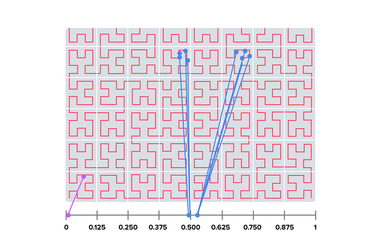
After comprehensive research on geo libraries, we landed on Google S2. S2 is based on Hilbert curve, a space-filling curve that preserves spatial locality: two points that are close on the Hilbert curve are close in physical space. Each smallest Hilbert curve clone is a cell, and 4 adjacent cells form a bigger cell, so it is a quadtree structure.

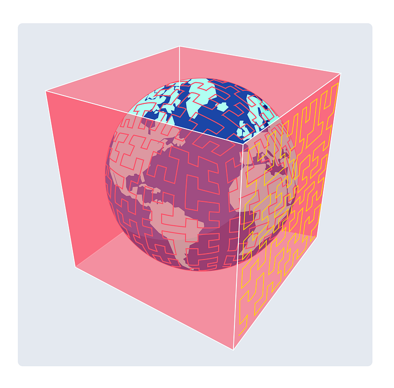
Now imagine there is a light in the center of the earth. It projects the globe’s surface to a tangerine cube where each face of the cube is filled with Hilbert curve, and each smallest cell represents an small area of the earth — that’s roughly how S2 does the mapping from an S2 cell. Notice that there will be distortion on the edge, especially on the corners — S2 does a non-linear transformation to make sure any projected cell’s actual size on the Earth’s surface is roughly the same. More details can be found in Google’s S2 slides.

S2 has the following advantages:

• Cells on the same level map to roughly the same size of area on Earth’s surface. Comparably, Geohash is very skewed when get near Earth’s poles.
• It’s a mature and stable library with support for main languages used by Tinder’s backend servers (Java and NodeJS).
• A 2D Hilbert curve is a quad tree, which makes aggregation quite easy. This is very convenient when calculating load score as you can maintain a load score in lower levels and aggregate to a higher level when needed.
• The library has built-in functionality to map a location (lat,long) => S2 cell, or cover a geographical area such as a polygon or circle with S2 cells.
• S2 has support for different-sized cells, ranging from square centimeters to miles.

S2 has cell levels ranging from Level-0 (33 million square miles) to Level-30 (1 square centimeter). After evaluating Tinder usage statistics, we found most users’ preferences are within a 50-mile range. As a result, S2 Level-7 (~45 miles) and Level-8 (~22.5 miles, see S2 statistics) are best suited for Tinder’s use case.

Now how do we create geoshards?

Notice that with S2, the entire globe can be mapped to a line of S2 cells. Now imagine each cell contains water proportional to their load score (e.g., load score 10 contains 10ml of water, the ones with load score 100.5 contain 100.5ml). You hold a container with size 1000ml, walk along the line of cells, and pour all the water in the cell that you passed by into the container, until you met a cell that contains enough water that will make the container overflow.

Now pour all the water out of the container into a bag and continue. Repeat the process until you reach the end of the line — you have made many bags, each bag is effectively a geoshard. Because S2 (and underlying Hilbert curve) preserves locality, the cells within a shard generated this way will be geographically together.

Given all the cells with precalculated load scores, the container size is the only factor that affects the sharding results.

If we enumerate all the possible container sizes, and calculate the standard deviation of each sharding configuration, the one with smallest standard deviation will be the most balanced geosharding configuration we are looking for.

The algorithm to find the best geoshard configuration looks like this for S2 Level-7(python-like pseudo code):

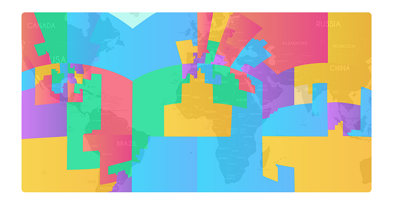
Then repeat the the same for S2 L8. At the end of the process, it will generate the best balanced geosharding configuration given the method. A visualization of generated geoshard mapping might look like the following graph. You can see Hilbert curve preserves locality really well, so geoshards are mostly physically together, and the geoshard is physically large for low load areas.

The generated geoshards store as a shard mapping json:

(Notice that S2 cell level 16 and above can be represented by either a LONG number id, or a string token. But different libraries in languages like Node/Java/Go generate different LONG id bytes for same cell, in the same time, the string token representation is consistent across these libraries, so we have chosen to use token to represent a S2 Cell.)

Using the geoshard mapping

There are two types of use cases that we need to consider:

• Indexing: given a user at (lat, long), map it to a geoshard
• Query: given a circle (lat, long, radius), get all the geoshards we need to query with

S2 libraries provides two functions:

• Given a location point (lat, long), return the S2 cell that contains it
• Given a circle (lat, long, radius), return all the S2 cells that are just enough to cover that circle

Notice that we already have a mapping from S2 cell to geoshard in the above shard mapping configuration. So:

• For an indexing request, the service first convert that to an S2 cell, then use the shard mapping to map the S2 cell to a geoshard
• For a query request, the service gets S2 cells that are just enough to cover the query circle using S2 library, then map all the S2 cells to geoshards using the shard mapping

The following image shows how the query mapping works. It is clear that this query with a 100 mile circle will only look up 3 out of 55 geoshards.

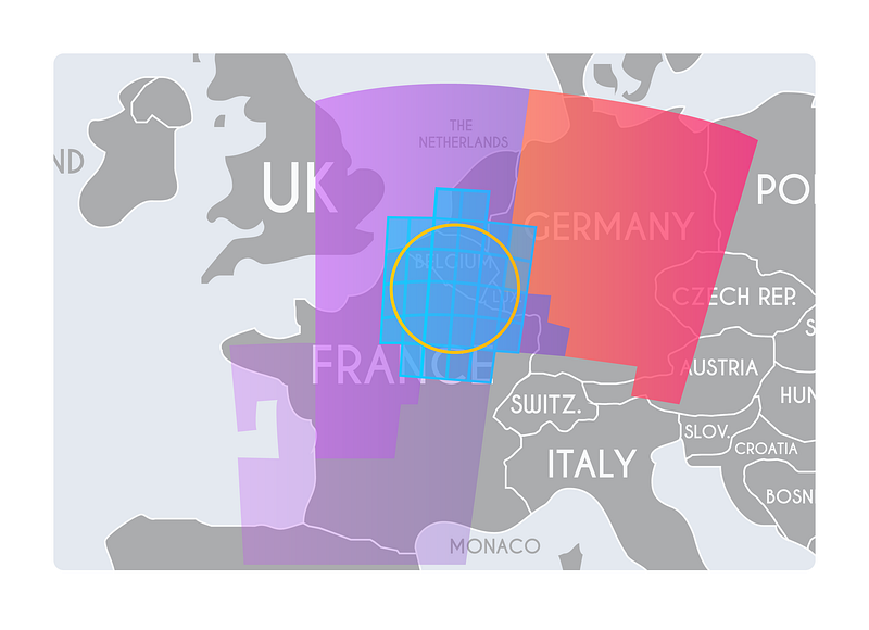
(Query: Circle => S2 Cells => geoshards)

About Resharding

In practice we have left enough room so there won’t be a need to reshard in years. But when needed, resharding can be done manually by running two parallel indices-sets with two shard mappings at the same time, then offline re-index all the existing docs to new geoshard indices, followed by a cutover and cleanup.

Takeaways

According to our measurement in production, the geosharded search index is capable of handling 20 times more computations compared to the single index setup. The great thing is that the method shown above can be applied to any computations that is location based and aggregatable.

Key takeaways:

• For a location-based service facing load challenge, consider geosharding
• S2 is a good library for geosharding, and Hilbert curves are awesome for preserving locality
• Consider how to measure load (load score) for better load balance between shards

Are you interested in building solutions to complex problems like these on a global scale? We are always looking for top talent and inventive problem solvers to join our engineering team. Check out our openings here!