Lifting 2D object detection to 3D in autonomous driving

Monocular 3D object detection predicts 3D bounding boxes with a single monocular, typically RGB image. This task is fundamentally ill-posed as the critical depth information is lacking in the RGB image. Luckily in autonomous driving, cars are rigid bodies with (largely) known shape and size. Then a critical question is how to effectively leverage the strong priors of cars to infer the 3D bounding box on top of conventional 2D object detection.

In contrast to conventional 2D object detection which yields 4 degrees of freedom (DoF) axis-aligned bounding boxes with center (x, y) and 2D size (w, h), the 3D bounding boxes in autonomous driving context generally have 7 DoF: 3D physical size (w, h, l), 3D center location (x, y, z) and yaw. Note that roll and pitch are normally assumed to be zero. Now the question is, how do we recover a 7-DoF object from a 4-DoF one?

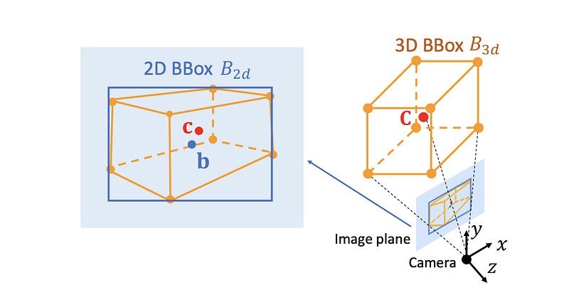
One popular way, proposed by the pioneering work of Deep3DBox (3D Bounding Box Estimation Using Deep Learning and Geometry, CVPR 2017) is to regress the observation angle (or local yaw, or allocentric yaw, as explained in my previous post) and 3D object size (w, h, l) from the image patch enclosed by the 2D bounding box. Both the local yaw and the 3D object size (which usually assumes a unimodal distribution with small variance around subtype mean) are strongly tied to object appearance and thus can be inferred from a cropped image patch. In order to fully recover the 7 DoF, we only need to infer the 3D location with three unknowns (x, y, z).

Luckily we can leverage the fact that the perspective projection of a 3D bounding box should fit tightly with its 2D detection window. This constraint forces that at least one cuboid vertex should project onto each of the four sides of the 2D box.

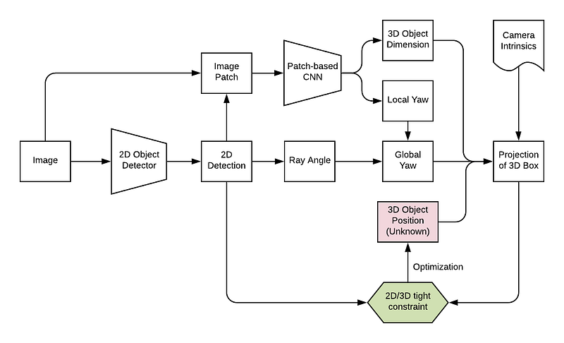
Following Deep3DBox’s footsteps, the following papers also explicitly follow the same formulation. Their contributions are to add different forms of a second stage to fine-tune the generated 3D cuboid, discussed in detail later in this post.

• FQNet: Deep Fitting Degree Scoring Network for Monocular 3D Object Detection (CVPR 2019)
• Shift R-CNN: Shift R-CNN: Deep Monocular 3D Object Detection with Closed-Form Geometric Constraints (TCIP 2019)
• Cascade Geometric Constraint: 3D Bounding Box Estimation for Autonomous Vehicles by Cascaded Geometric Constraints and Depurated 2D Detections Using 3D Results (ArXiv, Sept 2019)

The 2D/3D tight constraint

The four equations posed by the tight constraints can be written as follows. For each 2D bounding box parameterized by the coordinates of the top-left and bottom-right corners, (x_min, y_min, x_max, y_max), we have:

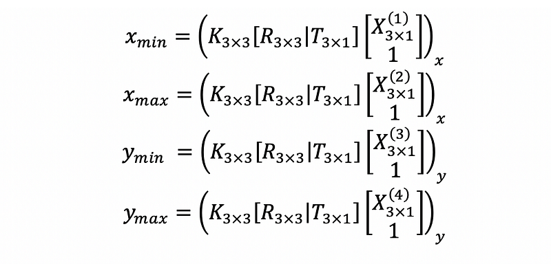
In the above equations, I have annotated the size of each matrix variable. X(1) to X(4) stand for the 4 selected vertices whose projection lies on the boundaries of the 2D bounding box. We will defer the selection of the 4 vertices later. The ()_x function takes the x component of the homogeneous coordinates, thus it is the ratio between the 1st and 3rd components. The same logic applies to the ()_y function. There are 3 unknowns and 4 equations, so it is an over-determined problem.

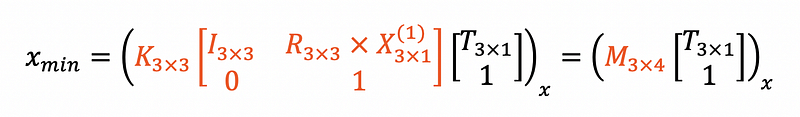
Note that in the above equations we want to solve for T. To make solving T a bit easier, it is useful to rewrite the above equation a bit. It is quite straightforward to show the two forms of formulations are equivalent. For simplicity, I am only showing the first equation here.

Solving the Equation Step by Step

Let’s rewrite the equation above and denote a large chunk of known parameters to matrix M with a shape of 3x4.

Written out in matrix formulation with Python numpy convention, it is

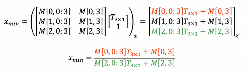
The above equation can be rearranged to the following

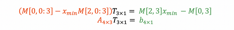
With four equations we can rewrite the left hand side as a 4x3 matrix A, and the right as a 4x1 matrix b. This over-determined linear equation can be solved by a least-square fitting by doing the Moore–Penrose pseudo-inversion (numpy.linalg.pinv in Python) of A.

Selection of Vertices and the Best Solution

One thing we did not talk about is how to select the 4 out of the 8 cuboid vertices that fall on the four sides of the 2D bbox. There is a long discourse in the original paper of Deep3DBox that under reasonable assumptions the number of plausible configurations can be reduced from 8⁴ to 64. Shift R-CNN has a similar conclusion but with slightly different reasoning to get to this number.

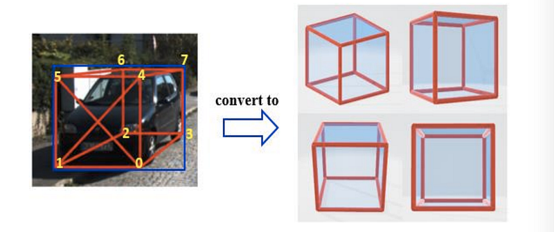
Personally, I found the explanation from Cascade geometric constraints the easiest to understand.

1. Pick one of the four lateral sides of a car cuboid as the side facing the viewer (e.g., 5-4-0-1 the front side of the car as the side facing the viewer in the figure above). Note that this only depends on the local yaw or observation angle.
2. Pick one of the four viewpoints as shown above (e.g., the left side example matches the top left viewpoint out of the four).
3. For the top two scenarios, the vertices touching the top and bottom sides of 2D bbox are fixed, but we still have four choices regarding which two vertices on the two vertical edges of the cuboid to select to conform to the left and right sides of the 2D bbox. For the bottom two scenarios, it is just the opposite — the vertices touching the left and right sides of the 2D bbox are fixed, but we have four choices regarding the top and bottom sides.

Thus in total, we have 4x4x4=64 plausible configurations.

Once the 64 configurations pass through the above 4 equations, the 64 solutions are ranked by fitting error (such as Deep3DBox, FQNet) or IoU score between the tightest bbox for the 8 projected vertices of the fitted cuboid and the 2D bbox (such as Shift R-CNN).

So far I found two implementations of this geometric constraint on Github, but they differ quite a bit, in terms of picking which vertices to use.

The drawbacks and the second stage

The above tight-constraint method infers 3D pose and position by placing the 3D proposal in 2D detection box compactly. This method sounds perfect in theory but it has two drawbacks: 1) It relies on accurate detection of 2D bbox — if there are moderate errors in the 2D bbox detection, there could be large errors in the estimated 3D bounding box. 2) The optimization is purely based on the size and position of bounding boxes, and image appearance cue is not used. Thus it cannot benefit from a large number of labeled data in the training set. To address this issue, there are several papers following up on the above workflow proposed by Deep3DBox and extend it with a second refinement stage.

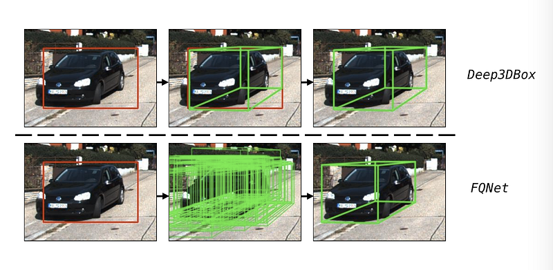
FQ-Net proposes to use the solved best fit as the seed position in 3D to densely sample 3D proposals. A neural network is then trained to tell the 3D IoU between the 3D proposal and the groundtruth by looking at an image patch with the 2D projection of the 3D proposal (green wireframe). The idea sounds wild but actually works.

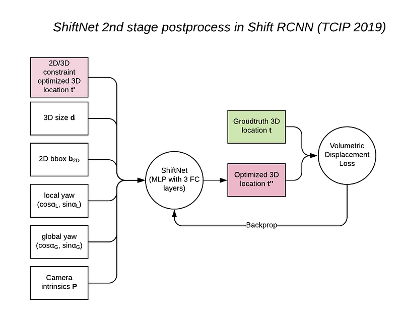
Shift R-CNN avoids dense proposal sampling by “actively” regressing the offset from the proposal. They feed all the known 2D and 3D bbox info into a fast and simple fully connected network called ShiftNet and refine the 3D location.

My verdict on Optimization

The optimization steps above, including those with a second stage, all assume the estimation of 3D size and local yaw is absolutely correct without any errors, and the errors the least square method minimizes are from the noise in the prediction of the 2D bounding box. This is a bit impractical and the most ideal way to do this is to allow some variation in the estimation of 3D size and local yaw as well and jointly optimize the error of the 7 DoF. This would make the constraint equations become non-linear and invalidate the above optimization steps with a beautiful closed form solution.

The Quick-and-Dirty Alternative

Besides the above tight constraint, there is actually a faster way to estimate the 3D position of the vehicle, simply based on the size of the 2D detection box or associated keypoints.

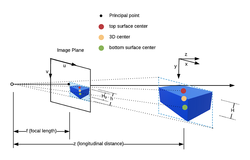
If we can tell in the image plane the projected positions of three keypoints on the 3D cuboid, we can estimate the distance via the simple principle of geometric similarity. Suppose we have the projection of the top surface, bottom surface and 3D cuboid center (as shown in the diagram above), we can get the ray angle between the ray going through principal point and the ray going through the 3D cuboid center. This ray angle is also called azimuth angle and is the key to connect local yaw and global yaw. To be exact, there should be two ray angle components, one in u- or x-direction and one in v- or y-direction.

Then according to the geometric similarity, we have f/z = H_p/H, where H_p is the v difference in image plane between the top and bottom surface center projection (in pixels), H is the height of 3D object (in meters), f is focal length (in pixels) and z is the longitudinal distance (in meters). With ray angles and z, we can perform coordinate transformation and recover the 3D position of the object.

This is exactly what Cascade Geometric Constraint does in inferring the initial 3D position (before feeding it to a Gauss-Newton algorithm to solve the constraint equations. Admittedly the equations above are convex and should have one global optimum and thus is insensitive to the initial condition, but this is another matter).

In addition, several other papers also use strong prior knowledge of the car size and keypoints to estimate depth.

• MonoPSR: Monocular 3D Object Detection Leveraging Accurate Proposals and Shape Reconstruction, CVPR 2019
• GS3D: An Efficient 3D Object Detection Framework for Autonomous Driving, CVPR 2019
• MonoGR2 Monocular 3D Object Detection via Geometric Reasoning on Keypoints

In particular, MonoPSR approximates distance with 2D bbox height then regresses the residual from RoIAligned feature. This essentially equates H_p and h in the figure above and could lead to some errors. GS3D approximated with 2D bbox height with a multiplicative factor of 0.93. This factor is obtained from analyzing the training dataset to reflect the difference between H_p and h in the figure above. MonoGR2 (pardon me for assigning a quick handle to this great work from Russia as they did not give a catchy name) regresses various keypoints on the car and approximated distance with the projected windshield height in the image. The 3D height of windshield comes from the matching 3D CAD models used in this study.

I personally prefer the method described in detail above by Cascade Geometric Constraint which is the most practical and reliable solution. But other methods work too if you truly want a “quick-and-dirty” estimate without going into the optimization business.

The brute-force alternative to geometric reasoning: Direct regression?

Besides the above tight constraint, geometric reasoning, I have also seen people directly regressing depth d or the disparity 1/d, such as CenterNet (Objects as Points — btw why isn’t it accepted at any top conference yet?) and SS3D: Monocular 3D Object Detection and Box Fitting Trained End-to-End Using Intersection-over-Union Loss. Obviously this works, but perhaps giving a better initialization with the above quick and dirty estimate will make it converge faster?

Takeaways

• Depth is hard to predict in monocular images, but it is critical in estimating accurate 7-DoF 3D cuboids with a monocular image. We can use strong visual cues and prior info such as the average size of the car to make educated guesses. This is how we humans do.
• We can solve four 2D/3D tight constraint equations, assuming 2D bounding boxes are accurate.
• We can get a quick and dirty estimate by leveraging the size of 2D bounding box or distances between known keypoints.
• We can also directly regress distance or disparity (although not widely popular)

References

[1] A Mousavian et al, Deep3DBox: 3D Bounding Box Estimation Using Deep Learning and Geometry (2017), CVPR 2017

[2] L Liu et al, FQNet: Deep Fitting Degree Scoring Network for Monocular 3D Object Detection (2019), CVPR 2019

[3] A Naiden et al, Shift R-CNN: Shift R-CNN: Deep Monocular 3D Object Detection with Closed-Form Geometric Constraints (2019), TCIP 2019

[4] J Fang et al, Cascade Geometric Constraint: 3D Bounding Box Estimation for Autonomous Vehicles by Cascaded Geometric Constraints and Depurated 2D Detections Using 3D Results (2019), ArXiv, Sept 2019

[5] J Ku et al, MonoPSR: Monocular 3D Object Detection Leveraging Accurate Proposals and Shape Reconstruction (2019), CVPR 2019

[6] B Li et al, GS3D: An Efficient 3D Object Detection Framework for Autonomous Driving (2019), CVPR 2019

[7] I Barabanau, MonoGR2: Monocular 3D Object Detection via Geometric Reasoning on Keypoints (2019), May 2019

[8] Y Zhou et al, CenterNet: Objects as Points (2019), ArXiv, April 2019

[9] E Jörgensen et al, SS3D: Monocular 3D Object Detection and Box Fitting Trained End-to-End Using Intersection-over-Union Loss (2019), ArXiv, June 2019