Generative Adversarial Network (GAN) for Dummies — A Step By Step Tutorial

The ultimate beginner guide for understanding, building, and training GANs with bulletproof Python code.

This article introduces everything you need to take off with generative adversarial networks. No prior knowledge of GANs is required. We provide a step-by-step guide on how to train GANs on large image datasets and use them to generate new celebrity faces using Keras.

“Generative Adversarial Network— the most interesting idea in the last ten years in machine learning” by Yann LeCun, VP & Chief AI Scientist at Facebook, Godfather of AI.

Although Generative Adversarial Network (GAN) is an old idea arising from the game theory, they were introduced to the machine learning community in 2014 by Ian J. Goodfellow and co-authors in the article Generative Adversarial Nets. How does a GAN work and what is it good for?

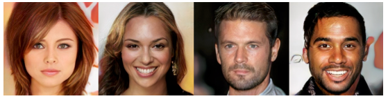
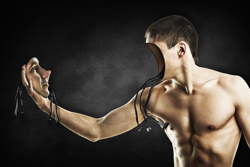
GANs can create images that look like photographs of human faces, even though the faces don’t belong to any real person.

We saw how to generate new photo-realistic images with a Variational AutoEncoder in our previous article. Our VAE was trained on the well-known Celebrity Faces Dataset.

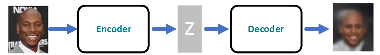
VAEs typically produce blurry and non-photorealistic faces. This is a motivation to built Generative Adversarial Networks (GANs).

In this article, we will look at how GANs offer a completely different approach to generating data that is similar to the training data.

The Game of Probabilities

Generating new data is a game of probabilities. When we are observing the world around us and collecting data, we are performing an experiment. A simple example is taking a photo of a celebrity's face.

This can be considered as a probabilistic experiment, with an unknown outcome X, also called a random variable.

If the experiment is repeated many times, we usually define the probability that the random variable X will get the value little x, as the fraction of times that little x occurs.

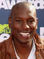
For example, we can define the probability that the face will be that of Tyrese, the famous celebrity singer.

All possible outcomes of such experiments build the so-called sample space, denoted Ω (all possible celebrity faces).

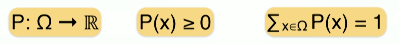
Therefore we can consider probability as a function that takes an outcome, i.e. an element from the sample space (a photo) and maps the outcome to a non-negative real number so that the sum of all these numbers equals 1.

We also call this a probability distribution function P(X). When we know the sample space (all possible celebrity faces) and the probability distribution (the probability of occurrence of each face), we have the full description of the experiment and we can reason about uncertainty.

You can refresh your knowledge of probabilities with our article below.

A celebrity-face probability distribution

Generating new faces can be expressed by a random variable generation problem. The face is described by random variables, represented through its RGB values, flatten into a vector of N numbers.

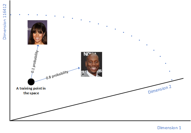
The celebrity faces are 218px height, 178px width with 3 color channels. Therefore each vector is 116412-dimensional.

If we build a space with 116412 (N) axes, each face will be a point in that space. A celebrity-face probability distribution function P(X) would map each face to a non-negative real number so that the sum of all these numbers for all faces equals 1.

Some points of that space are very likely to represent celebrity faces whereas it is highly unlikely for some others.

A GAN generates a new celebrity face by generating a new vector following the celebrity face probability distribution over the N-dimensional vector space.

In simple words, a GAN would generate a random variable with respect to a specific probability distribution.

How to generate random variables from complex distributions?

The celebrity-face probability distribution over the N-dimensional vector space is a very complex one and we don’t know how to directly generate complex random variables.

Luckily, we can represent our complex random variable by a function applied to a uniform random variable. This is the idea of the transform method. It first generates N uncorrelated uniform random variables, which is easy. It then applies a very complex function to that simple random variable! Very complex functions are naturally approximated by a neural network. After training the network will be able to take as input a simple N-dimensional uniform random variable and return another N-dimensional random variable that would follow our celebrity-face probability distribution. This is the core motivation behind generative adversarial networks.

Why Generative Adversarial Networks?

During each training iteration of the transform neural network, we could compare a sample of faces from our celebrity training set with a sample of generated faces.

Theoretically, we would compare the true distribution versus the generated distribution based on samples using the Maximum Mean Discrepancy (MMD) approach.

This would give a distribution matching error that could be used to update the network via backpropagation. This direct method is practically very complex to implement.

Instead of directly comparing both true and generated distributions, GANs solve a non-discrimination task between true and generated samples.

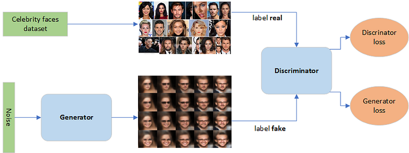
A GAN has three primary components: a generator model for generating new data, a discriminator model for classifying whether generated data are real faces, or fake, and the adversarial network that pits them against each other.

The generative part is responsible for taking N-dimensional uniform random variables (noise) as input and generating fake faces. The generator captures the probability P(X), where X is the input.

The discriminative part is a simple classifier that evaluates and distinguished the generated faces from true celebrity faces. The discriminator captures the conditional probability P(Y|X), where X is the input and Y is the label.

Training Generative Adversarial Networks

The generative network is trained to maximize the final classification error (between true and generated data), while the discriminative network is trained to minimize it. This is where the notion of adversarial networks arises from.

From the perspective of game theory, equilibrium is reached when the generator produces samples that follow the celebrity-face probability distribution and the discriminator predicts fake or not-fake with equal probability as if it would just flip a coin.

It is important that both networks learn equally during training and converge together. A typical situation occurs when the discriminative network becomes much better at recognizing fakes, causing the generative network to be stuck.

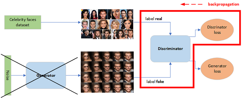
During discriminator training, we ignore the generator loss and just use the discriminator loss, which penalizes the discriminator for misclassifying real faces as fake or generated faces as real. The generator’s weights are updated through backpropagation. Generator’s weights are not updated.

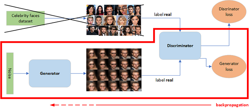
During generator training, we use the generator loss, which penalizes the generator for failing to fool the discriminator and generating a face that the discriminator classifies as fake. The discriminator is frozen during generator training and only generator’s weights are updated through backpropagation.

This is the magic that synthesizes celebrity faces using GANs. Convergence is often observed as fleeting, rather than stable. When you get everything right, GANs provide unbelievable results as demonstrated below.

Building and Training a DCGAN Model

In this section, we will go through all steps required to create, compile and train a DCGAN model for the celebrity faces dataset. Deep Convolutional Generative Adversarial Networks (DCGANs) are GANs that use convolutional layers.

The Discriminator

The discriminator can be any image classifier, even a decision tree. We use a convolutional neural network instead, with 4 blocks of layers. Each block includes a convolution, batch normalization, and another convolution with striding to downscale the image by a factor of two and another batch normalization. The result goes through average pooling, followed by a dense sigmoid layer which returns a single output probability.

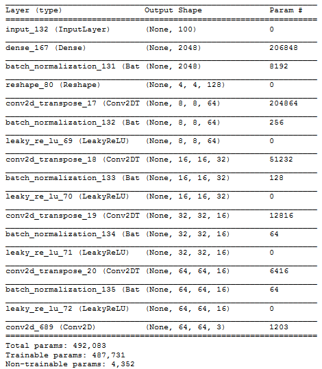
The Generator

The generator takes a noise vector of the latent dimension and generates an image. The shape of the image should be the same as the shape of the discriminator’s input (spatial_dim x spatial_dim).

The generator first upsamples the noise vector with the dense layer, in order to have enough values to reshape into the first generator block. The goal of the projection is to have the same dimension as the last block in the discriminator architecture. This is equivalent to 4 x 4 x number of filters in the last convolutional layer of the discriminator, as we will demonstrate later in this article.

Each generator block applies deconvolution to upsample the image and batch normalization. We use 4 decoder blocks and a final convolution layer to get a 3D tensor, which represents a fake image that has 3 channels.

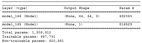
The GAN

The joined DCGAN is built by adding the discriminator on the top of the generator.

Before compiling the full setup, we have to set the discriminator model not to be trainable. This will freeze its weights and tell that the only part of the full network that needs to be trained, is the generator.

Although we compile the discriminator we don’t need to compile the generator model because we do not use the generator on its own.

This order ensures that the discriminator is updated at the right time and frozen when it has to be. Therefore if we train the whole model, it will just update the generator, and when we train the discriminator, it will only update the discriminator.

GAN Training

Now comes the hard and slow part: training a generative adversarial network. Because a GAN consists of two separately trained networks, convergence is hard to identify.

The following steps are executed back and forth allowing GANs to tackle otherwise intractable generative problems.

Step 1 — Select a number of real images from the training set.

Step 2 — Generate a number of fake images. This is done by sampling random noise vectors and creating images from them using the generator.

Step 3 — Train the discriminator for one or more epochs using both fake and real images. This will update only the discriminator’s weights by labeling all the real images as 1 and the fake images as 0.

Step 4 — Generate another number of fake images.

Step 5 — Train the full GAN model for one or more epochs using only fake images. This will update only the generator’s weights by labeling all fake images as 1.

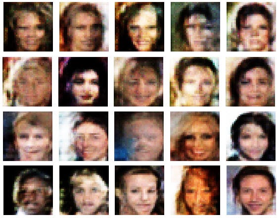
Above we can see that our GAN performed nicely. The generated faces look reasonable even if the photo quality is not so good as those in the CelebA training set. This is because we trained our GAN on reshaped 64x64 images, which became smaller and more blurry than the original 218x178.

Difference between VAE and GAN

Compared to the faces produced by Variational Autoencoder in our previous article, the ones generated by DCGAN look vivid enough to represent valid faces close enough to reality.

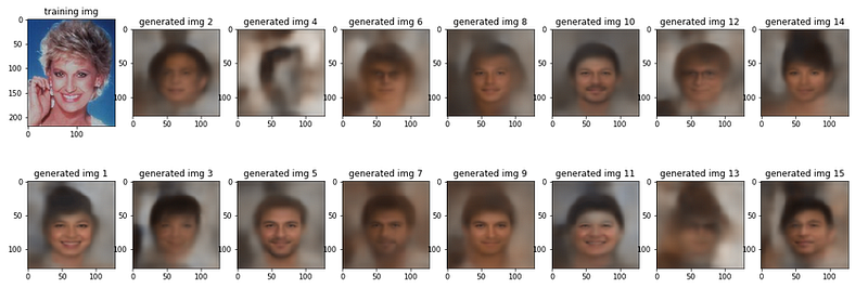
GANs are typically superior deep generative models as compared to VAEs. Although VAEs are bound to work in a latent space, they are easier and faster to train. VAEs can be considered semi-supervised learners because they are trained at minimizing a loss reproducing a certain image. A GAN, on the other hand, is solving an unsupervised learning problem.

Conclusion

In this article, I explained how generative adversarial networks are able to approximate the probability distribution of a large set of images and use it to generate photo-realistic images.

I provided working Python code that would allow you to build and train a GAN for solving your own task.

You can learn more about GANs with Google Developers or with Joseph Rocca’s article. Variational AutoEncoders are explored further in my article below.

Credits to Amber Teng from Towards Data Science for her editorial comments.

Thanks for reading. Stay safe. Stay well.