UNSUPERVISED LEARNING
Gaussian Mixture Models with Python
In this post, I briefly go over the concept of an unsupervised learning method, the Gaussian Mixture Model, and its implementation in Python.

The Gaussian mixture model (GMM) is well-known as an unsupervised learning algorithm for clustering. Here, “Gaussian” means the Gaussian distribution, described by mean and variance; mixture means the mixture of more than one Gaussian distribution.
The idea is simple. Suppose we know a collection of data points are from a number of distinct Gaussian models ( a Gaussian model is described by the mean scalar and the variance scalar for 1-d data and by the mean vector and variance matrix for N-d data), and we can know the probability of each data point belonging to one of the 2 Gaussian models if we know their density functions (as the example shown below). Then, we are able to assign the data point to the one specific model with the highest probability among the Gaussian mixture.
From the procedure described above, I believe you have already noticed that there are two most important things in the Gaussian mixture model. One is to estimate the parameters (as listed on the right of the figure above) for each Gaussian component within the Gaussian mixture and the other one is to determine which Gaussian component a data point belongs to. That’s why clustering is only one of the most important applications of the Gaussian mixture model, but the core of the Gaussian mixture model is density estimation.
To estimate the parameters that describe each Gaussian component in the Gaussian mixture model, we have to understand a method called Expectation-Maximization (EM) algorithm. The EM algorithm is widely used for parameter estimation when a model depends on some unobserved latent variables. The latent variable in the Gaussian mixture model is that describes which Gaussian component a data point belongs to. Since we only observed the data points, this variable is an unobserved latent variable.
In this post, I briefly describe the idea of constructing a Gaussian mixture model using the EM algorithm and how to implement the model in Python. When I was learning EM, my biggest problem was the understanding of the equations, so I will try my best to explain the algorithm without many equations in this post.
What does the EM algorithm really do in the GMM?
In short, the EM algorithm is for Gaussian parameter estimation. To better understand the concept, let’s start from the beginning.
Obviously, we have to understand a single Gaussian distribution before understanding a Gaussian mixture. Suppose we have a sequence of data points and each data point only has one feature (1-D dataset). We can plot the density of these data points along the axis of that feature.
For example, we want to describe the size of a bucket of Gala apples by measuring their diameters. Instead of knowing only the averaged diameters of the apples, we want to know the entire distribution of the sizes. So, we plot the distribution out as something below.
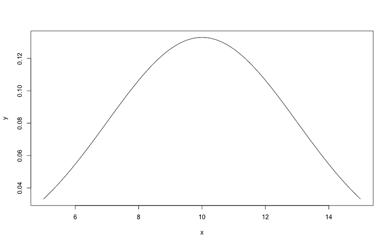
The density plot above can be also described by the equation below,
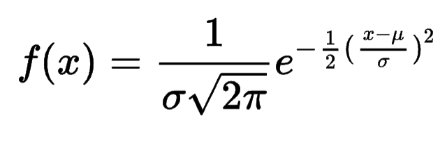
where μ is the mean and σ is the standard deviation.
Usually, we use the mean and variance to describe one Gaussian distribution. That’s easy, right?
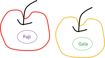
Next, suppose we have accidentally mixed one bucket of Gala and one bucket of Fuji apples together. We don’t have a fruit expert here, so no one around could separate Galas from Fujis. All we can do is still measure the sizes of the apples.
Are we still able to separate them? Theoretically, yes, if the Galas have real differences in size from the Fujis. To note, since we can only measure the size now, we should pray that this only feature can be good enough to separate the apples.
The situation described above is a real-world problem that a Gaussian mixture model clustering can be applied to. We would be very happy if the diameters of the apples follow two distinct Gaussian distributions as shown below,
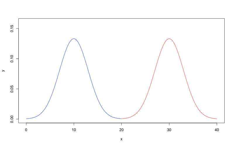
In such a case, we can simply apply a hard cutoff to separate the two kinds of apples. For example, larger (than 2 inches in diameter) ones are fuji 🍎 , and smaller (than 2 inches in diameter) ones are gala 🍏 .
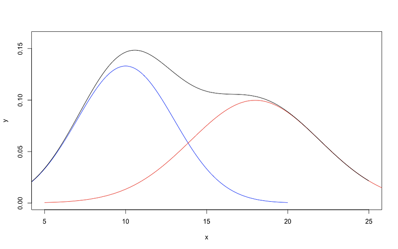
However, in most cases, we are going to observe a mixed distribution as shown below.
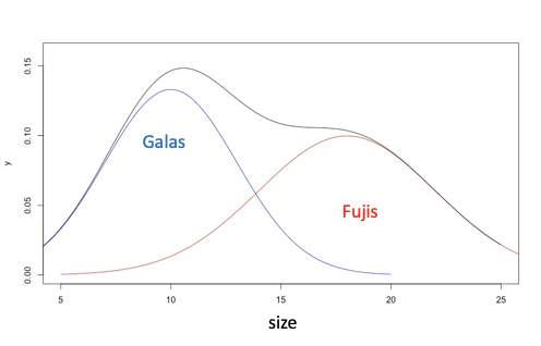
In the plot above, the black curve on top is our observed density of apple sizes, and it represents the two underlying Gaussian distributions that we cannot see. Let’s think about how to solve the problem in the most intuitive way.
(1) If we know the density function parameters (mean and variance) of the two distributions, for each apple, we can easily get the probability that it belongs to Fuji and also the probability that it belongs to Gala. If the probability of being a Fuji is larger than that of being a Gala, then it’s a Fuji, and vice versa. However, we don’t know the density function parameters.
(2) If we suddenly find that each apple actually already has the sticker on it, we can directly estimate the density function parameters for Fuji and Gala. But wait, if we already have the stickers, why should we bother doing everything? However, the real situation is that we don’t have the correct stickers because the fruit store owner’s son played with the apples and messed up the stickers.
What am I talking about? Do you think I’m crazy because point (1) and point (2) above are actually circular questions? We have to know one of them to solve the other one.
Actually, I was just describing one iteration of the EM algorithm. No worries, please let me explain it in detail.
The idea of the EM algorithm
The EM algorithm has a sequence of iterations of two major processes, the E-Step and the M-Step. E-Step estimates the latent variable, which is the probability of being a Fuji or Gala for each apple. This latent variable influences the data but is not observable. M-Step estimates the parameters of the distributions by maximizing the likelihood given the data. Likelihood describes how much a set of parameters matches the given data, for which we would like to get its maximal value (that best matches the given data, also called maximum likelihood estimation).
So, the real process of the EM algorithm should be something like,
EM EM EM EM EM EM EM…
Let’s get back to the specific question we are addressing.
The fruit store owner’s son helped us finish the initiation step of the EM algorithm, which randomly assigns labels (stickers) to the data points (apples). The idea is that since we cannot directly separate the data points, we just give a guess for the initialization. From now on, we should keep the little boy away from the apples.
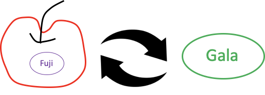
Ok, now let’s perform the E-step in the EM algorithm. Since we directly come from the initialization step, we already have the probability of being a Fuji or Gala for each apple. For an apple with a “Fuji” sticker, it has the probability of being a Fuji equal to 1, and the probability of being a Gala equal to 0.
However, if we come from a previous M-Step, we need to re-calculate the probability of being a Fuji or a Gala using the density function of the two Gaussians (estimated from the previous M-Step). If a previously labeled Fuji apple happens to have a larger probability to be a Gala than being a Fuji, then we replace the current sticker with a new “correct” Gala sticker on it. If there’s no disagreement between the previous label and the current probability, we keep the sticker unchanged.
Ok, now let’s perform the M-Step in the EM algorithm. No matter which iteration it is, we already have the initial/updated labels (stickers) on the apples. We can directly estimate the Gaussian parameters of Fuji and Gala distribution with the given labels. Basically, we estimate the Fuji Gaussian parameters based on only the apples with the sticker “Fuji” on them and then the Gala Gaussian parameters based on those with “Gala” on them. Theoretically speaking, we find the parameter set that maximizes the likelihood given the apple stickers.

And then, we repeat the two steps above over and over again until the assignment of the apples no more changes (strictly speaking, until the change in the likelihood function is very small).
That’s the full process of the EM algorithm in a real-world problem. How do you like the EM algorithm in the apple separation task? Is it hard? Did I use many equations? Not really, right?
Tips for better execution
If you really think about the apple separation task, you will realize there are a lot of realistic problems inside.
For example, the store owner’s little son just initiate the apple stickers randomly without even remembering what he did. So, will my apple separation task ends up very differently with different initial assignments of apple stickers? In addition, it should be hard to differentiate Gala from Fuji only by size, right?
The answer to the first question is yes for sure. Theoretically, it is not guaranteed that every random initiation will lead to the same final result in the EM algorithm for GMM. To address that, starting from some “initialization” that is not that random may be a good choice. If the little boy only played with 1/4 of the apples instead of messing up all the apple stickers, the current initiation probably will result in a much stable separation.
For the second question, it’s, of course, better to have more features. For example, the little boy not only played with the stickers of the apples but also bit each apple (Suppose he was able to record the flavor of each apple in a quantitative way). Then, for each apple, we have both the size and the flavor, which will probably lead to a better separation.
The Gaussian distribution with 2-D data can be visualized as an ellipse in the feature space. The following GIF shows the process of the EM algorithm for a Gaussian mixture model with three Gaussian components. You can imagine it as a task of separating Fuji, Gala, and Honeycrisp apples with the known size and flavor of each apple.
The X-axis and Y-axis in the GIF above could be the normalized size and the normalized flavor, respectively. You can see how the initialized three components gradually move to the specific apple clusters.
How to implement it in Python?
Compared to understanding the concept of the EM algorithm in GMM, the implementation in Python is very simple (thanks to the powerful package, scikit-learn).
import numpy as np
from sklearn.mixture import GaussianMixture
# Suppose Data X is a 2-D Numpy array (One apple has two features, size and flavor)GMM = GaussianMixture(n_components=3, random_state=0).fit(X)GaussianMixture is the function, n_components is the number of underlying Gaussian distributions, random_state is the random seed for the initialization, and X is our data. Here X is a 2-D NumPy array, in which each data point has two features.
After fitting the data, we can check the predicted cluster for any data point (apple) with the two features.
GMM.predict([[0.5, 3], [1.2, 3.5]])Sometimes, the number of Gaussian components is not that obvious. We can tune it by using AIC or BIC as the criteria (maybe further explained in future posts).
aic(X)
bic(X)
That’s it! The concept and implementation of GMM in Python. Hope it’s helpful.
If you think the article is too simple and general and you prefer more equations and mathematics, you can refer to the following excellent posts, here, here, and here.
References: