How I Build a GARCH Model for the Stock Market in Python

What are GARCH Models?

GARCH (Generalized Autoregressive Conditional Heteroskedasticity) models are a type of econometric models used to analyze and predict the volatility of financial time series, such as stock prices, bonds, interest rates, among others. Volatility refers to the measure of dispersion of returns of a financial asset over time.

GARCH models were initially proposed by Robert Engle in 1982 as an extension of ARCH (Autoregressive Conditional Heteroskedasticity) models. The main difference between ARCH and GARCH models lies in GARCH models allowing conditional volatility to evolve over time, whereas in ARCH models, volatility remains constant over time.

In a GARCH model, conditional volatility at time t is modeled as a function of the information available up to time t−1, and autoregressive terms are also included to capture temporal dependence patterns in volatility. These models are widely used in finance to estimate and predict asset price volatility, which can be useful in risk management, financial options valuation, and other financial applications.

Create one in python:

Part 1: Importing Packages

import numpy as np
import pandas as pd
import yfinance as yf
import matplotlib.pyplot as plt
import scipy.optimize as spop

Part 2: Specifying the Asset and Time Period

ticker = 'TSM'
start = '2018-12-31'
end = '2024-03-10'

Part 3: Downloading Data

prices = yf.download(ticker, start, end)['Close']

Part 4: Calculating Returns

returns = np.array(prices)[1:] / np.array(prices)[:-1] - 1

Part 5: Initializing GARCH Model Parameters

mean = np.average(returns)
var = np.std(returns)**2

Part 6: Defining the Negative Log-Likelihood Function

def garch_mle(params):
    mu = params[0]
    omega = params[1]
    alpha = params[2]
    beta = params[3]
    long_run = (omega / (1 - alpha - beta)) ** (1 / 2)
    resid = returns - mu
    realised = abs(resid)
    conditional = np.zeros(len(returns))
    conditional[0] = long_run
    for t in range(1, len(returns)):
        conditional[t] = (omega + alpha * resid[t - 1] ** 2 + beta * conditional[t - 1] ** 2) ** (1 / 2)
    likelihood = 1 / ((2 * np.pi) ** (1 / 2) * conditional) * np.exp(-realised ** 2 / (2 * conditional ** 2))
    log_likelihood = np.sum(np.log(likelihood))
    return -log_likelihood

This part defines the garch_mle() function that calculates the negative log-likelihood of the GARCH model. It takes the model parameters as input and returns the negative log-likelihood.

Part 7: Maximizing Likelihood

res = spop.minimize(garch_mle, [mean, var, 0, 0], method='Nelder-Mead')
params = res.x

The minimize() function from scipy.optimize is used to maximize the negative log-likelihood and obtain the optimal parameters for the GARCH model.

Part 8: Extracting Optimal Parameters

mu = res.x[0]
omega = res.x[1]
alpha = res.x[2]
beta = res.x[3]
log_likelihood = -float(res.fun)

Part 9: Calculating Realized and Conditional Volatility for Optimal Parameters

long_run = (omega / (1 - alpha - beta)) ** (1 / 2)
resid = returns - mu
realised = abs(resid)
conditional = np.zeros(len(returns))
conditional[0] = long_run
for t in range(1, len(returns)):
    conditional[t] = (omega + alpha * resid[t - 1] ** 2 + beta * conditional[t - 1] ** 2) ** (1 / 2)

Part 10: Printing Optimal Parameters

print('GARCH model parameters')
print('')
print('mu ' + str(round(mu, 6)))
print('omega ' + str(round(omega, 6)))
print('alpha ' + str(round(alpha, 4)))
print('beta ' + str(round(beta, 4)))
print('long-run volatility ' + str(round(long_run, 4)))
print('log-likelihood ' + str(round(log_likelihood, 4)))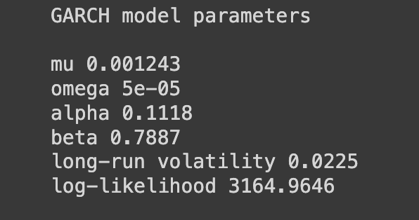

Interpretation of each parameter:

1. mu (μ): This parameter represents the mean of the stochastic process modeling the returns. In this case, the value of μ is approximately 0.001243. It indicates that, on average, positive returns are expected.
2. omega (ω): It is the coefficient associated with the constant variance in the GARCH model. A small value of ω (5e-05 in this case, meaning 5 × 10^-5) indicates that most of the variability of returns is explained by autoregressive and conditional volatility terms, not by a constant variance.
3. alpha (α): It is the coefficient associated with the volatility shock term in the GARCH model. It indicates the sensitivity of conditional volatility to the squared error in the previous step. In this case, α is approximately 0.1118, suggesting that past volatility shocks have a moderate effect on future volatility.
4. beta (β): It is the coefficient associated with the previous conditional volatility in the GARCH model. It represents the persistence of volatility. A high value of β (0.7887 in this case) indicates that volatility in one time period significantly affects volatility in the next period.
5. Long-run volatility: This is the long-term volatility of the stochastic process modeled by the GARCH. It is calculated as the square root of ω divided by the square root of 1 minus the sum of α and β. In this case, the long-run volatility is approximately 0.0225.
6. Log-likelihood: The log-likelihood is a measure of how well the model fits the data. In this case, the value of the log-likelihood is 3164.9646. A higher value indicates a better fit of the model to the observed data.

Part 11: Visualizing the Results

plt.figure(1)
plt.rc('xtick', labelsize=10)
plt.plot(prices.index[1:], realised)
plt.plot(prices.index[1:], conditional)
plt.show()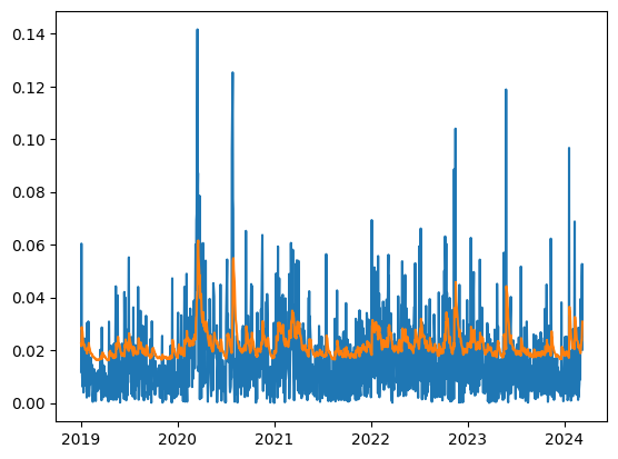

Conclusion:

GARCH models are powerful and widely used tools in the analysis of financial time series. They allow for modeling and forecasting the volatility of asset prices, which is crucial for risk management, financial options valuation, and other financial applications. By capturing the heteroskedastic nature of financial data, GARCH models offer a more accurate representation of volatility dynamics compared to simpler models. However, it’s important to note that GARCH models have assumptions and limitations that should be considered when interpreting results. Overall, GARCH models have proven to be valuable tools for understanding and managing volatility in financial markets.