Getting Started

Fundamentals of Generative Adversarial Networks

GANs — Illustrated, explained and coded

Synthetic handwritten digits generated by a GAN. In this tutorial, we’ll create our own GAN that can generate digits just like this, as well as the code to create this animation above. Read on!

Introduction

In 2014, a then-unknown Ph.D. student named Ian Goodfellow introduced Generative Adversarial Networks (GANs) to the world. GANs were unlike anything the AI community had seen, and Yann LeCun described it as “the most interesting idea in the last 10 years in ML”.

Since then, much research effort have poured into GANs, and many state-of-the-art AI applications such as NVIDIA’s hyper-realistic face generator are derived from Goodfellow’s work on GANs.

Author’s note: All images and animations in this article are created by the author. If you would like to use the images for educational purposes, kindly drop me a note in the comments. Thank you!

What are GANs, and what can they do?

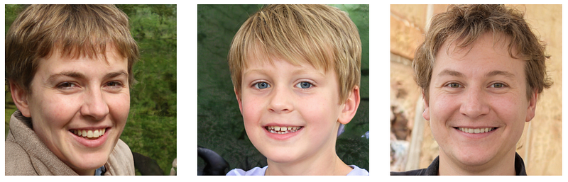
At a high level, GANs are neural networks that learn how to generate realistic samples of the data on which they were trained on. For example, given photos of handwritten digits, GANs learn how to generate realistic photos of more handwritten digits. More impressively, GANs can even learn to generate realistic photos of human beings, such as those below.

Human faces generated by a GAN. None of the above faces above are real. Source: https://thispersondoesnotexist.com/

So how do GANs work? Fundamentally, GANs learn the distribution of the subject of interest. For example. GANs that are trained on handwritten digits learn the distribution of the data. Once the distribution of the data has been learnt, the GAN can simply sample from the distribution to generate realistic images.

Distribution of the data

To solidify our understanding of the distribution of the data, let’s consider the following example. Suppose that we have the following 6 images below.

Each image is a grayish box, and for simplicity, let’s assume that each image consists of just 1 pixel. In other words, there is just one grayish pixel in each image.

Now, suppose that each pixel has a possible value between -1 and 1, where a white pixel has a value of -1 and a black pixel has a value of 1. The 6 gray images would therefore have the following pixel values:

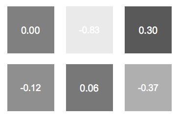
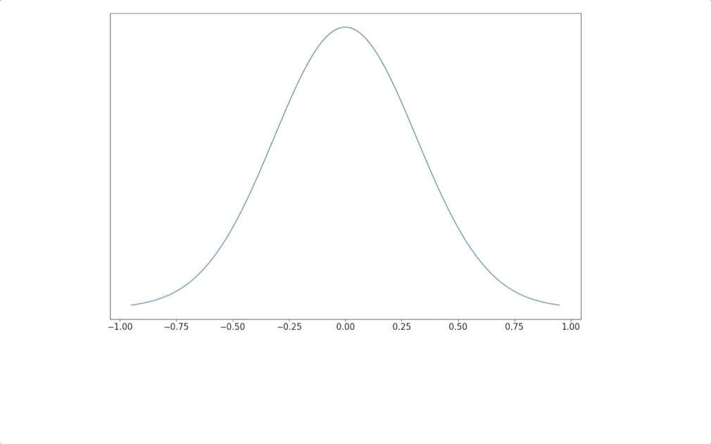
What do we know about the distribution of the pixel values? Well, just by inspection, we know that most pixel values are around 0, with few values nearing the extremities (-1 and 1). We can therefore assume that the distribution is a gaussian, with a mean of 0.

Note: With more samples, it is trivial to derive the gaussian distribution of this data by calculating the mean and standard deviation. However, this is not our focus since it is intractable to calculate the data distribution of complex subjects, unlike in this simple example.

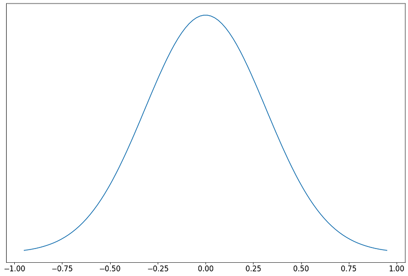
Underlying distribution of our pixel is a gaussian distribution with mean of 0

This data distribution is useful because it allows us to generate more gray looking images, just like the 6 above. To generate more similar images, we can randomly sample from the distribution.

10 pixels drawn randomly and independently from a gaussian distribution. Notice that most pixel values are near the mean (0), with few outliers at the extremities (-1 and 1).

While it may be trivial to figure out the underlying distribution of gray pixels, computing the distribution of cats, dogs, cars or any other complex object is often mathematically intractable.

How then, do we learn the underlying distribution of complex objects? The obvious answer is to use neural networks. Given sufficient data, we can train a neural network to learn any complex function, such as the underlying distribution of the data.

Generator — The Distribution Learning Model

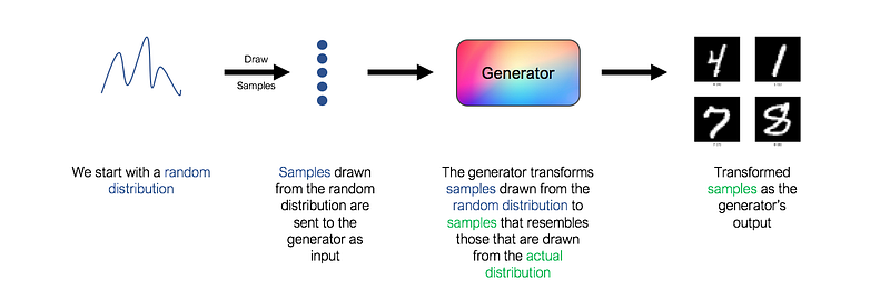
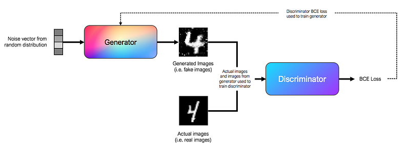
In a GAN, the generator is the neural network that learns the underlying distribution of the data. To be more specific, a generator takes as input a random distribution (also known as ‘noise’ in GANs literature), and learns a mapping function that maps the input to the desired output, which is the actual underlying distribution of the data.

However, notice that a key component is missing in the architecture above. What loss function should we use to train the generator? How do we know if the images generated actually resemble actual handwritten digits? As always, the answer is ‘use a neural network’. This second network is known as the discriminator.

Discriminator — The Generator’s Adversary

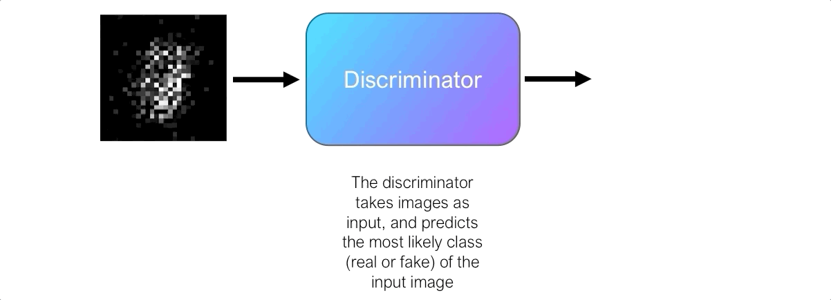
The discriminator’s role is to judge and assess the quality of output images from the generator. Technically, the discriminator is a binary classifier. It accepts images as input, and outputs a probability that the image is real (i.e. actual training image), or fake (i.e. from the generator).

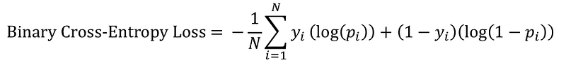
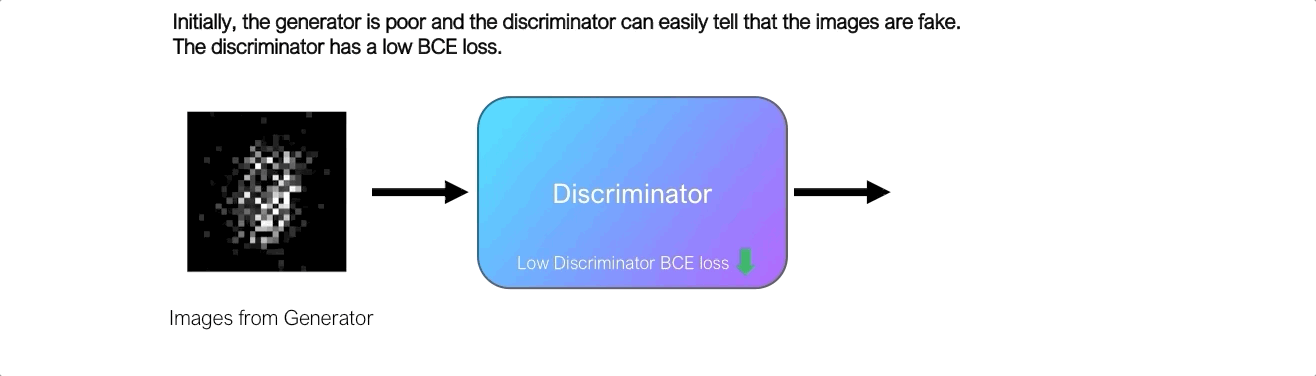
Initially, the generator struggles to produce images that look real, and the discriminator can easily distinguish real and fake images without making too many mistakes. Since the discriminator is a binary classifier, we can quantify the performance of the discriminator using the Binary Cross-Entropy (BCE) Loss.

The discriminator’s BCE loss is an important signal for the generator. Recall earlier, that by itself the generator doesn’t know if the generated images resemble the real images. However, the generator can use the discriminator’s BCE loss as a signal to obtain feedback for its generated images.

Here’s how it works. We send images output by the generator to the discriminator and it predicts the probability that the image is real. Initially, when the generator is poor, the discriminator can easily classify the images as fake, resulting in a low BCE loss. However, the generator eventually improves and the discriminator starts to make more mistakes, misclassifying the fake images as real, which results in a higher BCE loss. Therefore, the discriminator’s BCE loss signals the quality of image output by the generator, and the generator seeks to maximize this loss.

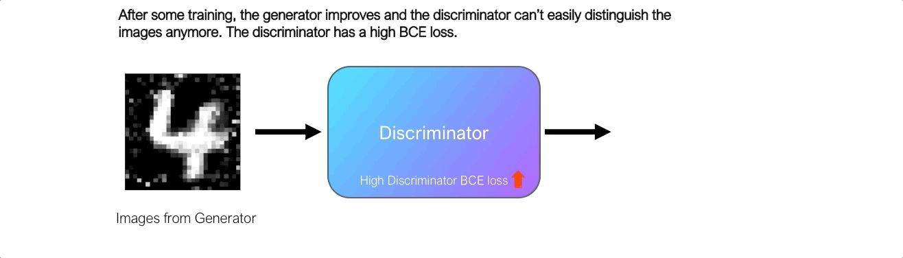
The discriminator’s BCE loss is an indicator of the quality of the images output by the generator

As we can see from the animation above, the BCE loss from the discriminator is correlated to the quality of images produced by the generator.

The generator uses the discriminator’s loss as an indicator of the quality of its generated images. The objective of the generator is to tune its weights such that the BCE loss from the discriminator is maximized, effectively ‘fooling’ the discriminator.

Training the Discriminator

But what about the discriminator? So far, we assumed that we have a perfectly working discriminator right from the start. However, this assumption isn’t true and the discriminator requires training as well.

Since the discriminator is a binary classifier, its training procedure is straightforward. We’ll provide a batch of labelled real and fake images to the discriminator, and we’ll use the BCE loss to tune the weights of the discriminator. We train the discriminator to identify real vs fake images, preventing the discriminator from being ‘fooled’ by the generator.

GANs — A tale of two networks

Let’s put everything together now and see how GANs work.

By now, you know that GANs consist of two interlinked networks, the generator and the discriminator. In conventional GANs, generators and discriminators are simple feedforward neural networks.

What’s unique to GANs is that the generator and discriminator are trained in turns, adversarial to one another.

To train the generator, we use a noise vector sampled from a random distribution as input. In practice, we use a 100 length vector drawn from a gaussian distribution as the noise vector. The input is passed through a series of fully connected layers in the feedforward neural network. The output of the generator is an image, which in our MNIST example, is a 28x28 array. The generator passes its output to the discriminator, and uses the discriminator’s BCE loss to tune its weights, with the aim of maximizing the discriminator’s loss.

To train the discriminator, we use labelled images from the generator, as well as actual images as input. The discriminator learns to classify the images as real or fake, and is trained using the BCE loss function.

In practice, we train the generator and discriminator in turns, one after another. This training scheme is akin to a two-player minimax adversarial game, as the generator aims to maximize the discriminator’s loss, and the discriminator aims to minimize its own loss.

Creating our own GAN

Now that we understand the theory behind GANs, let’s put it into practice by creating our own GAN from scratch using PyTorch!

First of all, let’s bring in the MNIST dataset. The torchvision library allows us to get the MNIST dataset easily. We’ll do some standard normalizing to the images before flattening the 28x28 MNIST images to a 784 tensor. This flattening is required as the layers in the network are fully connected layers.

Next, let’s write the code for the generator class. From what we have seen earlier, a generator is simply a feedforward neural network that accepts a 100 length tensor and outputs a 784 tensor. In a generator, the size of the dense layers are usually doubled after each layer (256, 512, 1024).

That was easy wasn’t it? Now, let’s write the code for the discriminator class. The discriminator is also a feedforward neural network that accepts a 784 length tensor, and outputs a tensor of size 1 , denoting the probability that the input belongs to class 1 (real image). Unlike the generator, we halve the size of the dense layers after each layer(1024, 512, 256).

Now, we’re going to create a GAN class that encompasses both the generator and the discriminator class. This GAN class will contain the code for training the generator and discriminator in turns, according to the training scheme that we have discussed earlier. We’re going to use PyTorch Lightning for this, in order to simplify our code and reduce boilerplate code.

The code is commented above and it’s pretty self explanatory given what we have discussed so far. Notice how modularizing our code using PyTorch Lightning makes it look so neat and readable!

We can now train our GAN. We’ll train it using the GPU, for 100 epochs.

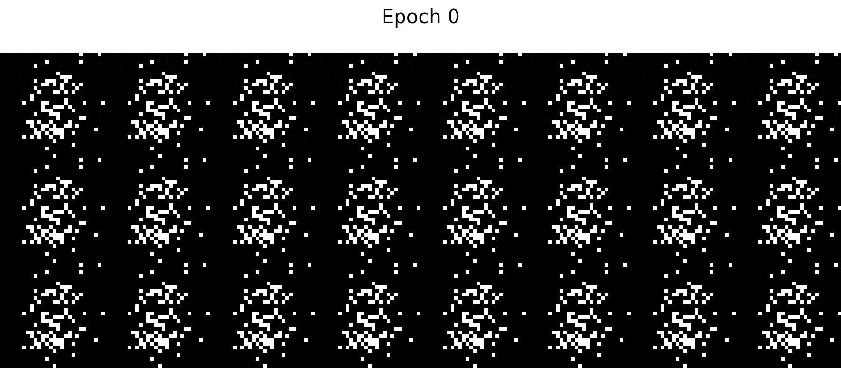
Visualizing The Generated Images

All that’s left now is to visualize the generated images. In the training_epoch_end() function from our GAN class above, we saved the images output from the generator after each training epoch into a list.

We can visualize these images by plotting them on a grid. The code below randomly selects 10 images generated after the 100th training epoch and plots them on a grid.

And this is the output:

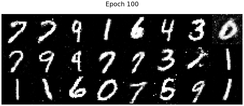
That’s pretty good! The output resembles real handwritten digits. Our generator has definitely learnt how to fool the discriminator.

Finally, as promised, we’ll create the animation shown at the top of the post. Using theFuncAnimation function in matplotlib , we’ll animate the images on the plot, frame by frame.

What’s Next?

Congrats! You made it to the end of this tutorial. I hope you’ve enjoyed reading this as much as I’ve enjoyed writing this. Fortunately for us, this is not the end of our journey. Shortly after the original GAN was introduced by Goodfellow, the scientific community poured in huge efforts in this area, which led to a proliferation of GAN-based AI models.

I’m beginning a series of tutorials just like this, where I illustrate, explain and code up the different variations of GANs, including important ones such as Deep Convolutional GAN (DCGAN) and Conditional GAN (CGAN). Be sure to follow me (if you haven’t already!) to be informed whenever the new tutorials are out.

Other Resources

The code here can be found in my Github repository as well. I will be updating this repository continuously to include other variations of GANs in the future.