Fundamentals of Deep Learning -Neural Networks

Deep Learning, many of us using this tool to solve the most complicated problems even without understanding it. Tensorflow framework and Keras Interface makes life easy for everyone. But it is necessary to know the basic concepts of Neural Networks to make your solutions more precise. Let me share my understandings.

Why Neural Networks are important?

Imagine that we have a problem, the bank gave all of the transaction details such as customer name, age, bank balance, retired or not, transactions and so on. And asks us to build a model which can predict the Number of Transactions a customer will make next year. Problems seem very simple. Many of us would think of a linear Regression to solve this problem.

y = b + w1x1 + w2x2 + w3x3 + ……………………. + wnxn

But, look at this equation of linear regression. The result is the sum of the individual parts. it doesn’t find the interaction between any of the features. To be more clear, linear regression can map the features to results but they cannot find the relationships between features.

This is why Neural Networks are important. Because in many problems features interact with each other in different ways. The neural network has the ability to find these interactions between features.

What is Forward Propagation?

It is a simple technique used in Neural Networks to find Interactions between Features. For example, imagine we have the Number of Children of a customer Number of Accounts a customer has. The results we need to predict is the number of transactions.

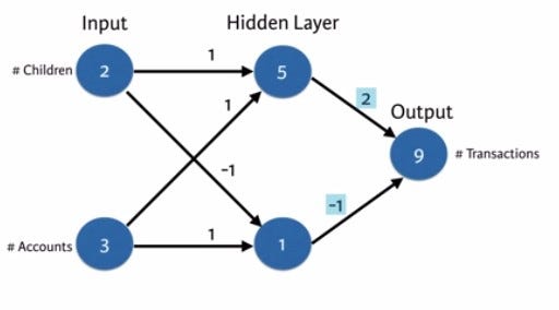
Above picture explains how forward propagation works. We have two inputs, in NN each input represented by Neurons (nodes), such collection of neuron known as a layer. Always our input layer has the dimension of our input size and out layer has the dimension of outputs we are expecting. Each successive layers between input and output layers are known as hidden layers.

The values for each successive layers’ neurons are calculated by the multiplying the input nodes with the appropriate weights. The image itself explains it clearly. Let us see a simple code example,

import numpy as np 

input_data = np.array([2,3])

#node_0 and node_1 gives the weights of hidden layer and output gives the weights to calculate the output
weights = {
  'node_0': np.array([1,1]),
  'node_1': np.array([-1,1]),
  'output': np.array([2,-1])}

node_0_value = (input_data * weights['node_0']).sum()
node_1_value = (input_data * weights['node_1']).sum()

hidden_layer = np.array([node_0_value, node_1_value])
print(hidden_layer)

output = (hidden_layer * weights['output']).sum()
print(output)

What is Activation Function and why we need them?

Multiplying inputs with weights and adding them is too straight forward. It is not obvious that our data will always have a linear relationship between them. There may be nonlinearities between data(features), so we need to capture those nonlinearities to increase the ability of NN. We use Activation functions to do that.

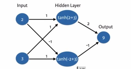
Activation function can be any function, but there are some activation functions which in use such as tanh, relu, softmax and many others. I am not going to go in details of how to choose them. We pass the multiplied values to this activation function and store the returned values in corresponding nodes. Normally we define the activation function when defining the layers. Every node in a single layer will use the same Activation function. Let's see a simple code example for how these functions work,

The rectified linear activation function (called ReLU) has been shown to lead to very high-performance networks. This function takes a single number as an input, returning 0 if the input is negative, and the input if the input is positive.

def relu(input):
      '''Define your relu activation function here'''
      output = max(input, 0)
      
      # Return the value just calculated
      return(output)

# Define predict_with_network()
def predict_with_network(input_data_row, weights):

      # Calculate node 0 value
      node_0_input = (input_data_row * weights['node_0']).sum()
      node_0_output = relu(node_0_input)

      # Calculate node 1 value
      node_1_input = (input_data_row * weights['node_1']).sum()
      node_1_output = relu(node_1_input)

      # Put node values into array: hidden_layer_outputs
      hidden_layer_outputs = np.array([node_0_output,   node_1_output])
      
      # Calculate model output
      input_to_final_layer = (hidden_layer_outputs * weights['output']).sum()
      model_output = relu(input_to_final_layer)
      
      # Return model output
      return(model_output)

# Create empty list to store prediction results
results = []
input_data_row = np.array([2,3])
weights = {
  'node_0': np.array([1,1]),
  'node_1': np.array([-1,1]),
  'output': np.array([2,-1])}

for input_data_row in input_data:
    # Append prediction to results
    results.append(predict_with_network(input_data_row, weights))4
print(results)

Deeper Networks

So far we have worked with one hidden layer, but in real scenarios, we will have many hidden layers with a different number of nodes. Deep networks internally build increasingly sophisticated representations of patterns in the data using each successive layers. This helps to partially eliminate the need for feature engineering and makes life easier for ML engineers. Below codes show an example of Deep Network with two hidden layers,

input_data = np.array([3,5])
weights = {'node_0_0': np.array([2,4]),
      'node_0_1': np.array([4,-5]),
      'node_1_0': np.array([-1,2]),
      'node_1_1': np.array([1,2]),
      'output'  : np.array([2,7])
      }

#use the relu funtion wrote in previous example
def predict_with_network(input_data):
     # Calculate node 0 in the first hidden layer
     node_0_0_input = (input_data * weights['node_0_0']).sum()
     node_0_0_output = relu(node_0_0_input)

     # Calculate node 1 in the first hidden layer
     node_0_1_input = (input_data * weights['node_0_1']).sum()
     node_0_1_output = relu(node_0_1_input)

     # Put node values into array: hidden_0_outputs
     hidden_0_outputs = np.array([node_0_0_output, node_0_1_output])
     
     # Calculate node 0 in the second hidden layer
     node_1_0_input = (hidden_0_outputs * weights['node_1_0']).sum()
     node_1_0_output = relu(node_1_0_input)

     # Calculate node 1 in the second hidden layer
     node_1_1_input = (hidden_0_outputs * weights['node_1_1']).sum()
     node_1_1_output = relu(node_1_1_input)

     # Put node values into array: hidden_1_outputs
     hidden_1_outputs = np.array([node_1_0_output, node_1_1_output])

     # Calculate model output: model_output
     model_output = (hidden_1_outputs * weights['output']).sum()
     
     # Return model_output
     return(model_output)

output = predict_with_network(input_data)
print(output)

The weights are adjusted during the training to achieve expected model performance, which is called Optimization. Stay tuned to know more details about optimization techniques such as Gradient descent and backpropagation. Follow me to getting instant notifications and updates.