From Pixels to Photorealism: The Art of 3D Gaussian Splatting

Imagine watching fireflies glow in a dark field at night. Each firefly emits a light that is brightest at its position and fades as you move away. These glowing areas can be represented using 3D Gaussians. When combined, they create a field of glowing blobs similar to a technique called Gaussian Splatting.

What is Gaussian Splating?

Gaussian Splatting is a powerful technique in computer vision and graphics used for 3D image reconstruction. It involves projecting 2D image features (such as key points or pixel intensities) into 3D space, represented as a Gaussian distribution centered at each 3D position. These Gaussians are then combined to form a continuous 3D representation of the scene, which is particularly useful for real-time radiance field rendering, enabling photorealistic scenes from a limited number of images.

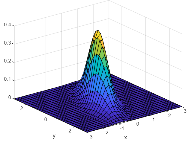
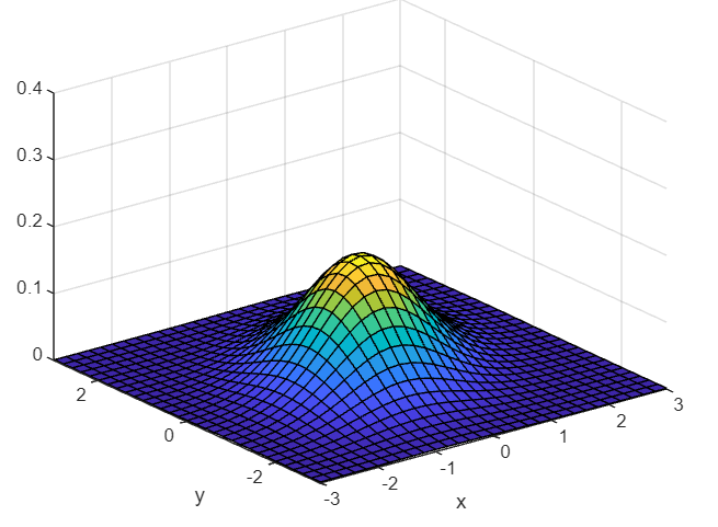
The Math Behind Gaussian Splatting

The Gaussian Splatting process involves calculating the Gaussian function for each keypoint or pixel in the image. This function resembles a smooth, bell-shaped curve, similar to a hill when plotted on a graph. The center of the bump is the most influential, with the influence decreasing smoothly as you move away from the center.

The Gaussian function is defined by the equation:

where (𝑥,𝑦,𝑧) are the coordinates of the keypoint or pixel, (𝑋,𝑌,𝑍)are the coordinates in 3D space, and 𝜎 is the standard deviation controlling the spread of the Gaussian.

In detail,

which shows how the Gaussian value decreases as you move away from the center (x,y,z).

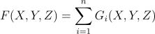
Summing up these Gaussians results in a smooth, continuous 3D surface approximating the shape defined by the n key points.

Example

Let us understand this concept more clearly by a simple example. Consider defining 4 keypoints for a 2D rectangle and assigning a constant depth value to lift these keypoints into 3D space. Applying a Gaussian function creates smooth splats centered at each keypoint. These are then combined to form a 3D representation. This process helps transform a simple 2D shape into a 3D model using Gaussian Splatting, illustrating how individual points contribute to the overall 3D structure.

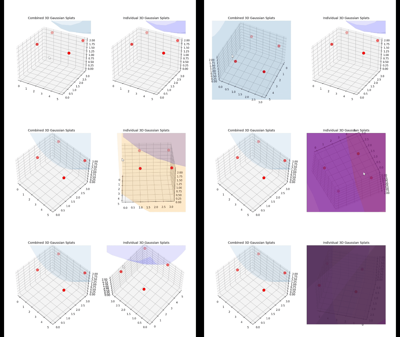
When visualizing the above scenario, we get the above result. Here, the animation shows each Gaussian splat with a distinct color, highlighting the contribution of each key point on the right. On the left, a smooth, continuous 3D shape is represented by an isosurface formed by the combined 3D Gaussian splats from all key points defined by the same “blue color”.

Rendering with 3D Gaussian Splatting

Rendering in 3D Gaussian involves projecting these Gaussians onto the image plane. Each Gaussian’s contribution is computed based on its projection and its parameters like covariance matrix, and opacity (𝛼) allowing for flexible optimization.

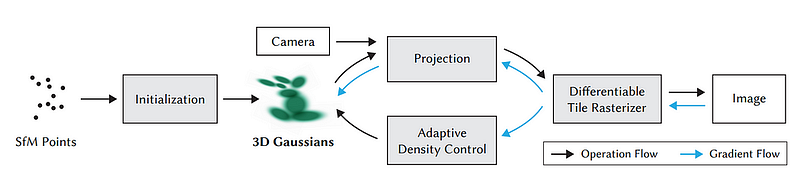
The architecture of 3D Gaussian for real-time radiance field rendering can be given below. The method starts with a set of images of a static scene and corresponding camera calibrations from Structure from Motion (SfM) that produces a sparse point cloud. From these points, a set of 3D Gaussians is created, defined by its position, covariance matrix, and opacity (𝛼). This approach results in a compact 3D scene representation, capable of efficiently representing fine structures using anisotropic volumetric splats. Then these Gaussian parameters are optimized while adaptively controlling Gaussian density. The efficiency is enhanced by a tile-based rasterizer that enables 𝛼-blending of splats to create the final image.

In Gaussian Splatting, the scene is represented as a collection of Gaussians, each associated with color and opacity. The color of the radiance field is represented via spherical harmonics. The radiance field is thus approximated by these Gaussians:

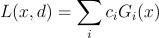
where 𝑐 represents the color of the 𝑖-th Gaussian, and G​(x) is its value at point 𝑥.

Mathematically,

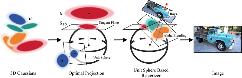
The projection of a Gaussian onto the image plane involves an affine transformation of the Gaussian function from the world coordinate system to the camera coordinate system via a viewing transformation matrix.

where 𝑢 and 𝑣 are coordinates on the image plane, and 𝑆 is the transformed covariance matrix in the camera coordinate system

After the transformation, the contributions of all Gaussians are composited. The colors and opacities are blended based on their projected positions and weights to produce a final image. The parameters of the Gaussians (mean, covariance, color, and opacity) can be optimized to better fit the scene’s radiance field. Optimization techniques, such as Gradient Descent, can minimize the error between the rendered image and the ground truth.

Here is an example of rendering of 3D Gaussians generated from the sparse point clouds.

Practical Example: Modeling a Tree

Let’s create a 3D model of a tree, representing its trunk and leaves, and project it onto a 2D plane:

trunk_params = [(0, 0, i, 0.1, 0.1, 0.5, 0, 0, 0) for i in np.linspace(-2, 2, 10)]

# Parameters for the leaves (a cluster of Gaussians around the top of the trunk)
leaves_params = [(np.random.uniform(-0.5, 0.5), np.random.uniform(-0.5, 0.5), np.random.uniform(1.5, 2),0.3, 0.3, 0.3, 0, 0, 0) for _ in range(50)]

# Combine parameters
all_params = trunk_params + leaves_params

Now create a 3D Gaussian function utilizing the above equation

def gaussian_3d(x, y, z, mux, muy, muz, sx, sy, sz, rho_xy, rho_xz, rho_yz):
    X, Y, Z = np.meshgrid(x, y, z, indexing='ij')
    X_shifted = X - mux
    Y_shifted = Y - muy
    Z_shifted = Z - muz
    
    # Create the covariance matrix
    covariance_matrix = np.array([
        [sx**2, rho_xy * sx * sy, rho_xz * sx * sz],
        [rho_xy * sx * sy, sy**2, rho_yz * sy * sz],
        [rho_xz * sx * sz, rho_yz * sy * sz, sz**2]
    ])
    
    inv_covariance_matrix = np.linalg.inv(covariance_matrix)
    
    # Compute the exponent component-wise
    exponent = (X_shifted**2 * inv_covariance_matrix[0, 0] +
                Y_shifted**2 * inv_covariance_matrix[1, 1] +
                Z_shifted**2 * inv_covariance_matrix[2, 2] +
                2 * X_shifted * Y_shifted * inv_covariance_matrix[0, 1] +
                2 * X_shifted * Z_shifted * inv_covariance_matrix[0, 2] +
                2 * Y_shifted * Z_shifted * inv_covariance_matrix[1, 2])
    
    gaussian = np.exp(-0.5 * exponent)
    
    return gaussian

Finally, generate and add each Gaussian to the volume. Summing along the Z-axis projects it onto the 2D plane, which is then normalized to create the given output.

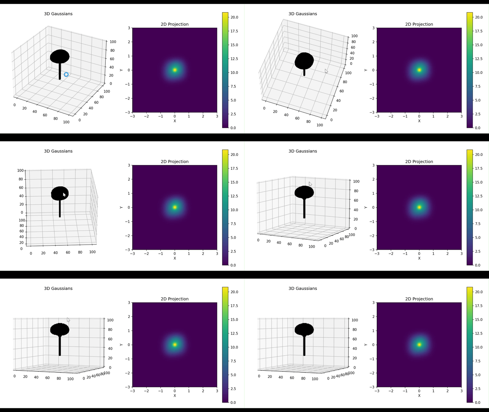
By integrating Gaussian Splatting, we can effectively create and render photorealistic 3D models from 2D images, enhancing our capability in fields like computer vision, graphics, and augmented reality.

Reference

1. Kerbl, B., Kopanas, G., Leimkühler, T., & Drettakis, G., “3D Gaussian Splatting for Real-Time Radiance Field Rendering”, arXiv:2308.04079, 2023
2. Huang, L., Bai, J., Guo, J., & Guo, Y., “Optimal Projection for 3D Gaussian Splatting”,arXiv.2402.00752v2, 2024

3. Hugging Face, Article