From Messy to Neat with Python Pandas

A practical tutorial

Real life data is usually messy. It does not come in the most appealing format for analysis. A substantial amount of time for a project is spent on data wrangling.

We can start data analysis and infer meaningful insights only after the data is in an appropriate format. Luckily, Pandas provides numerous functions and techniques that expedite the data cleaning process.

In this article, we will take a dataset about obesity rates which looks messy and convert it to a nice and clean format. Each step involves a different Pandas function so it will also be like a practical tutorial.

Let’s start by importing the libraries and reading the dataset.

import numpy as np
import pandas as pd

df = pd.read_csv("/content/data.csv")

df.shape
(198, 127)

The dataset contains 198 rows and 127 columns. Here is a screenshot of the first 5 rows and columns.

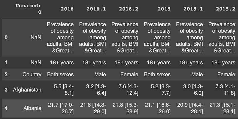
Except for the first 3 rows, the columns contain obesity rates from 1975 to 2016.

df.columns[-5:]  # last 5 columns

Index(['1976.1', '1976.2', '1975', '1975.1', '1975.2'], dtype='object')

The first 3 rows do not seem to be inline with the following lines. Let’s check the values in these rows. The unique function returns the unique values in a row or column.

# First row
df.iloc[0,:].unique()

array([nan,        'Prevalence of obesity among adults, BMI ≥ 30 (age-standardized estimate) (%)'],       dtype=object)

# Second row
df.iloc[1,:].unique()

array([nan, '18+  years'], dtype=object)

The first 2 rows seem to define the entire dataset instead of individual columns. There is only one unique value and a NaN value in the first 2 rows so we can drop them.

The drop function can be used to drop rows or columns depending of the axis parameter value.

df.drop([0,1], axis=0, inplace=True)

We specify the rows to be dropped by passing the associated labels. The inplace parameter is used to save the changes in the dataframe.

There are 3 columns for each year which contain the obesity rate for males, females, and average of the two. Since we can easily obtain the average from the male and female values, it is better to drop the columns that indicate the average value.

One way is to pass a list of columns to the dropped. It is kind of a tedious way because there are 42 columns to be dropped. Pandas offers a more practical way which allows us to select the every third item from a list.

The df.columns method returns the indices of the columns. We can select the every third item starting from index 1 as follows:

df.columns[1::3]
Index(['2016', '2015', '2014', '2013', '2012', '2011', '2010', '2009', '2008', '2007', '2006', '2005', '2004', '2003', '2002', '2001', '2000', '1999', '1998', '1997', '1996', '1995', '1994', '1993', '1992', '1991', '1990', '1989', '1988', '1987', '1986', '1985', '1984', '1983', '1982', '1981','1980', '1979', '1978', '1977', '1976', '1975'],       
dtype='object')

We can pass this list to the drop function.

df.drop(df.columns[1::3], axis=1, inplace=True)

Here is how the dataframe looks like now:

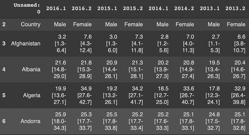
We already know 1 means male and 2 means female. Thus, we can rename the first column as “Country” and drop the first row.

df.rename(columns={'Unnamed: 0': 'Country'}, inplace=True)

df.drop([2], axis=0, inplace=True)

The dataset is in a wide format. It will easier to analyze in a long format in which the years are represented in one column instead of separate columns.

The melt function is just for this tasks. Here is how we can convert this dataframe from wide to long format.

df = df.melt(
   id_vars='Country', var_name='Year', value_name='ObesityRate'
)

df.head()

Each year-country combination is represented in a separate row.

The obesity rate column includes an average value and a value range. We need to separate them and represent with numbers. For instance, we can have three columns which are the average, lower limit, and upper limit.

The functions under the str accessor can be used to extract the lower and upper limit.

df['AvgObesityRate'] = df.ObesityRate.str.split(' ', expand=True)[0]

df['LowerLimit'] = df.ObesityRate.str.split(' ', expand=True)[1].str.split('-', expand=True)[0].str[1:]

df['UpperLimit'] = df.ObesityRate.str.split(' ', expand=True)[1].str.split('-', expand=True)[1].str[:-1]

We first split the obesity rate column at space character which separates the range from the average value. We then split the range at the “-” character and use indexing to extract the limit values.

We can now drop the obesity rate column since we have extracted each piece of information.

df.drop('ObesityRate', axis=1, inplace=True)

df.head()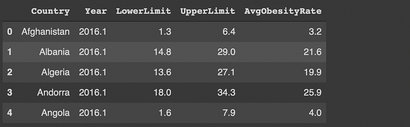

The final step is to add the gender information. In the current format, the year column represents the gender (1 is male and 2 is female). We can separate the 1s and 2s from the year and replace them accordingly.

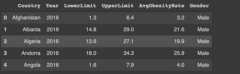
df['Gender'] = df['Year'].str.split('.', expand=True)[1].replace({'1': 'Male', '2': 'Female'})

df['Year'] = df['Year'].str.split('.', expand=True)[0]

We have used the split function as in the previous step. Using a dictionary in the replace function makes it possible to replace multiple values at once.

Here is the final version of the dataset:

Conclusion

We took a dataset in a messy format and convert it to a neat and clean format. The information in the dataset remains the same but the format matters to perform efficient data analysis.

Pandas is both a data manipulation and data analysis library. In this article, we have focused on the data manipulation part. The flexible and versatile functions of Pandas expedite the data wrangling process.

Thank you for reading. Please let me know if you have any feedback.