Fractionally Differentiated Features to Preserve Memory in Stationary Time Series

How to Properly Preprocess Data for Machine Learning Trading Bots

The method is described from Advances in Financial Machine Learning by Marcos López de Prado.

Motivation

The problem of stationarity is often found in time-series data. In this article, I want to give you an intuition on the problem and how to solve it properly without losing you in too many details. If you are interested to dive deep into the topic, I suggest you read: Advances in Financial Machine Learning by Marcos López de Prado. It is really a great book if you are interested in applying Machine Learning in Finance.

A Machine Learning algorithm needs the data to be stationary so it can work properly. Before throwing the definition of stationarity I want to give you an intuition about it. Let’s say that we have the price of an asset over a period of time. The training data has prices that vary within the interval [90$; 100$]. The algorithm will learn that everything that is around 90$ is cheap and everything that is around 100$ is expensive. Because the price of an asset moves its mean price over time, the test split will have the price within [100$; 110$]. Now the algorithm will think that the asset is always expensive, even though that is not true because now 100$ is the lowest point. This will mess with the algorithm and it will probably make very strange predictions.

Now let's see the definition of stationarity: A time series has stationarity if a shift in time doesn’t cause a change in the shape of the distribution. Basic properties of the distribution like the mean , variance and covariance are constant over time.

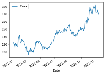
As an example, we can see in the figure below the prices of Apple from 2021 to 2022. It doesn’t look very stationary right?

Also, in this article, I will present to you why the standard integer differentiation is not good enough for memory preservation.

Theoretical Demonstration

If you are interested in how the method is demonstrated you may like this section.

Initial formulation

First, let’s define some variables:

X = data
B = backshift operator
k = number of observations that we take from the past
d = scaling factor

Now let’s define the backshift operator:

Now I have to remind you about the binomial series, this is very important:

As a final step we will apply the binomial series formula to the defined variables:

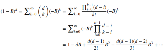
Now let’s break down what this means. It is not as scary as it looks. Let’s take for example 1 — dB . We take the data point from the current moment t minus the data point from the previous moment t-1 scaled by a factor of d . In the classic integer differentiation method d=1 . So basically, we just take data points from the past, scale them with some fancy formulas, and in the end add them all together.

Weights

The hard part of the demonstration has passed. Let’s define what our time series X looks like. It is a set of data points from the past relative to the k variable:

We compute every current data point relative to past observations with the following formula:

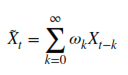
This is where everything adds up. The weights are the fancy scaling values computed a few steps above:

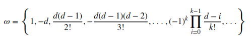
So basically, for every current point, we take k points from the past, multiply each of them by their corresponding weight w , and in the end, add them together. As an example, when d=1 the weights will be w = {1, -1, 0, 0, ....} , this is the particular case we know as integer differentiation. For d=2 the weights will be w = {1, -2, 1, 0, .....} etc.

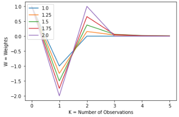
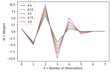
One interesting thing happens when d is not an integer. In that case, the weights will not cancel out when k > d, but they will slowly converge to the value of 0. We can see this behavior more clearly in the figures below

In this figure, we can see that for d = 0 & d = 1 the weights are 0 when k > d . But, for d float values within the interval, we can see that their value is not 0, but it slowly converges towards 0.

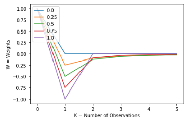
Let’s see this applied in more examples for a better understanding of the concept:

Those are the steps that we use for a single point in time. To make the time series stationary, we have to repeat this process for every point in time.

Iterative Estimation of the Weights

To apply the formula described above we need to have two things: X and W , where both are considered to be vectors/arrays/lists ( what works for you).

X is just a slice of length k from our time series. We can easily compute W iteratively with the following formula:

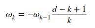
When k=0 the value of w=0 . From now on we go recursively until the weight will be smaller than a certain threshold. Usually, it is better to go in the past until a certain threshold is reached than to choose a fixed kvalue. Otherwise on what criteria would you choose k? In our examples we will use a threshold of 0.001. But you can always tweak this value for your convenience. Below I attached the Python code that computes the weights:

def get_weights(d: int, thres: float) -> np.ndarray:
    w, k = [1.], 1
    
    while True:
        w_ = -w[-1] / k * (d - k + 1)
        if abs(w_) < thres:
            break
        w.append(w_)
        k += 1
        
    return np.array(w[::-1]).reshape(-1, 1)

Ok, but how do we know the best value of d? This is what the next section is all about.

How to Find the Value of d?

We are almost done with our algorithm. To find the best d value we will use the Augmented Dickey-Fuller unit root test to identify stationarity. It is not within the scope of this article to explain the method. All you need to know is that it helps us to identify if a time series is stationary or not. You can find an implementation of it at the statsmodels Python package.

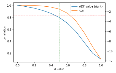
Also, we will test for the correlation between the initial time series and the processed one to see how well it preserves memory. The lower the ADF value is, the better. The lower the value, the best it tests for stationarity. But this value is relative, it doesn’t tell us much. That is why we will use the 95% confidence value associated with its ADF value . This is equivalent with a p value smaller than <5% .

We will only use the Apple prices as examples in this article. So to find the best d value we have to pick the intersection between the ADF value curve and the red dotted line, as we see in the figure below. The green line reflects that more exactly it happens for d=0.5 . We can see that for d=0.5the preprocessed time series is still highly correlated with the original one. This means that our task of memory preservation succeeded.

Implementation of how we computed the graph from above:

def search_parameters(data: pd.DataFrame) -> pd.DataFrame:
    parameters = pd.DataFrame(columns=['ADF value', 'p value', 'lags', 'nObs', '95% conf', 'corr'])
    for d in np.linspace(0, 1, 11):
        df1 = data[['Close']].resample('1D').last()
        df2, _ = frac_diff_fixed(df1, d, size=5)
        corr = np.corrcoef(df1.loc[df2.index, 'Close'], df2['Close'])[0, 1]
        df2 = adfuller(df2['Close'], maxlag=1, regression='c', autolag=None)
        
        parameters.loc[d] = list(df2[:4]) + [df2[4]['5%']] + [corr]
    
    ax = parameters[['ADF value', 'corr']].plot(secondary_y='ADF value')
    ax.set_xlabel('d value')
    ax.set_ylabel('correlation')
    plt.axhline(parameters['95% conf'].mean(), linewidth=1, color='r', linestyle='dotted')
    
    d_value = find_d_value(parameters)
    if d_value is not None:
        plt.axvline(d_value, linewidth=1, color='g', linestyle='dotted')
    
    return parameters, d_value

def find_d_value(parameters: pd.DataFrame) -> float:
    conf_95 = parameters['95% conf'].mean()
    for d_value, row in parameters.iterrows():
        if row['ADF value'] <= conf_95:
            return d_value
        
    return None

How to apply the weights on our original time series:

def frac_diff(data: pd.DataFrame, d: float, thres=1e-3) -> Tuple[pd.DataFrame, np.ndarray]:
    w = get_weights(d, thres)
    width = len(w) - 1
    
    df = {}
    for name in data.columns:
        column_data = data[[name]].fillna(method='ffill').dropna()
        differentiated_column_data = pd.Series(dtype=np.float32)
        for end_iloc in range(width, column_data.shape[0]):
            start_loc = column_data.index[end_iloc - width]
            end_loc = column_data.index[end_iloc]
            if not np.isfinite(data.loc[end_loc, name]):
                # Exclude NaNs
                continue
            differentiated_column_data[end_loc] = np.dot(w.T, column_data.loc[start_loc:end_loc]).item()
        df[name] = differentiated_column_data.copy(deep=True)
    df = pd.concat(df, axis=1)
    
    return df, w

Now Let’s See Some Results

We will download our data with the yfinance Python package. We get everything from the start of 2021 at a frequency of 1d . The function bellow will return a Pandas DataFrame with the Apple stock prices & volume:

data = yfinance.download(
            tickers=['AAPL'],
            start='2021-01-01',
            end=None,
            interval='1d',
            auto_adjust=True,
            prepost=False
        )

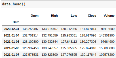
This is what our data looks like:

We will work with log prices, so we have to run the following command:

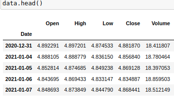
data = data.apply(np.log)

Now, this is how our data looks:

Let’s apply the fractional differentiation algorithm to our Apple price time series with the d value we found:

d_value = 0.5
data_frac_diff, w_frac_diff = frac_diff(data, d_value)
plot_weights(d_range=[d_value], n_plots=1, size=len(w_frac_diff))

This is what the weights look like:

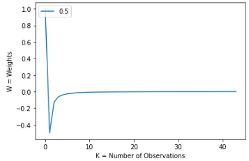
We can see that from k~=4 all the weights are closer and closer to 0. But they are not 0, which is important. They keep going until k~=40. This is one factor why the correlation is still so strong between the preprocessed and original time series. Let’s see what the last 5 weights look like:

[[-0.00121631]
 [-0.00126629]
 [-0.0013198 ]
 [-0.00137718]
 [-0.00143885]]

Finally, we will see the final results:

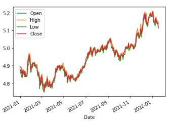
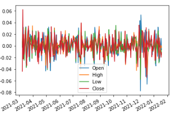
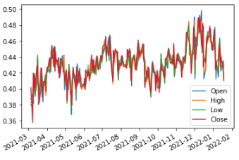
As we discussed in this article the original time series is clearly not stationary. In Fig 2 we plotted the data processed with the integer differentiation method. We can visually see that even though, it is stationary, there isn’t much information left. Probably, only the outliers can still be noticed. Fig 3 reflects our method in which we can definitely see the same trends as in the original time series. We can see that mostly, we have the same mean and variance in any shift of time. It is not yet 100% stationary, if we would like that we could increase the d value and see what happens.

You can find the full implementation on my GitHub.

Conclusion

We can definitely notice the need for our data to be stationary. Also, we have seen that with integer differentiation the signal is lost and the data looks more like noise. Therefore, I consider that the fractional differentiation method should be used widely in the Financial Machine Learning field.

Thank you for reading my article! If you liked it hit the 👏 button so other people can see the article. I would also appreciate feedback from you so I can improve my presentation skills.

Do not hesitate to reach me via the following :

• Follow me on Medium
• Connect and reach me on LinkedIn
• Write me at my mail address: [email protected]