[Fractional Calculus Demystified: Part 2] Riemann-Liouville Derivatives

Disclaimer: you’ll find the Fundamental Theorem of Calculus to be actually quite genius after this article

How would we even begin to define a fractional calculus? Hopefully you’ve taken a look at part 1 of this article series to recall the Fundamental Theorem of Calculus. The fundamental theorem tells us that, for appropriate functions, it will be true that

Cool! We have a relationship between the integral of a function and its derivative. The way to begin to understand a fractional derivative is actually first through fractional integration! Let’s look at a curious formula sometimes dubbed the Cauchy iterated integral formula. Note, our functions are real-valued so this is not exactly the Cauchy integral formula we may be familiar with from complex analysis.

Iterated and Fractional Integrals

We can consider first what happens when you iterate two integrals

It turns out we can express this as a single integral! The way we do this is by switching the two integrals. In order to do this, we pick up the assumption that f is integrable in both s and t. In practice, this assumption isn’t actually very restrictive since your favorite functions tend to be integrable anyway. But the question remains as to how exactly to switch these integrals. Take a look at the region in question:

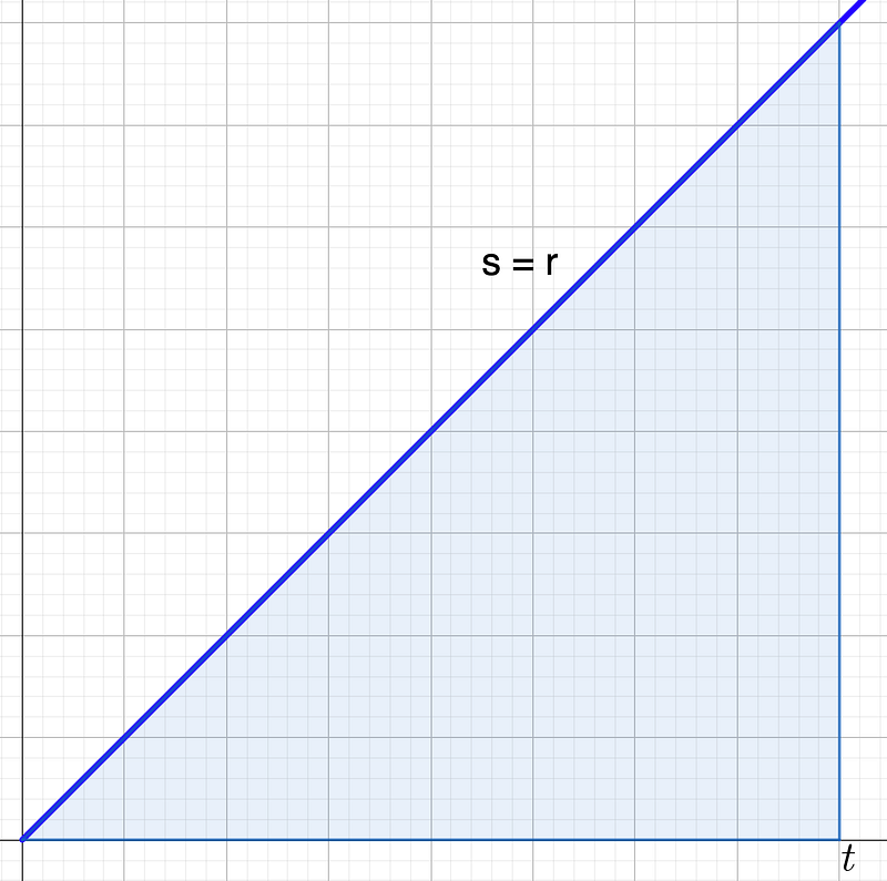
Here, the integral is telling us to go first in the r (vertical) direction and then in the s (horizontal) direction. When we switch the integrals, we still want to capture this very same area but switching the directions. That, is we will go horizontal first and then vertical. In the horizontal direction, our integral is going to travel from the diagonal line s = r to the right hand border s = t. Then, we tell the integral to form the triangle by going from 0 to t in the r direction. That is,

In the last equality, we evaluated the ds integral. Since f is a function of r, it would not go inside the innermost integral and we can just evaluate that as the length of the interval (t-r). That’s great and dandy, but how does this help us? Notice that iterating an integral turned into a linear multiplier!

Can we keep doing this sort of thing? Yes! If you keep iterating integrals, you can always write it as a single integral while paying the price in the form of a polynomial multiplier! The general formula reads as follows:

The (n-1)! term is picked up the integration that has to happen over and over again. Now, this formula works for counting number n. For more details on these calculations, check out this great video (at around minute 13) by Dr. Joel Rosenfeld. However, what’s to say that this factor cannot be, say, 1/2? It turns out that, inspired by this formula, we can figure out a definition for a fractional integral!

So, replace n by a real number α between 0 and 1. We can generalize the factorial term with its natural generalization, the Gamma function (for now, just know that it’s a number and that it is convenient to have it there) and arrive at the fractional integral of f

Neat, right? Staring at this definition while tilting your head should immediately bring up a million questions in your mind. I’ll make a list for some immediate ones:

1. Is this object even well-defined?
2. If α is between 0 and 1, isn’t α-1 negative? If so, then really we are looking at a fraction right?
3. If we are looking at a fraction, should we be careful with dividing by 0? I hear that’s a big no no in math.
4. Does this expression have anything to do with derivatives? I only see integrals.
5. Are there other ways to define a fractional integral?

The short answer to all these questions is Yes. Well, okay, with some technicalities involved. My hope is to further explore these technicalities in subsequent parts of our series.

But wait! I’ll give one (of many) answers to the fourth question posed. We can define the Riemann-Liouville (R-L) derivative of order α of a function f as follows:

Ah, finally the fractional derivative promised land. Feels good to have made it here, right? Notice an interesting thing happening here. This is phrased as a derivative of an integral. In other words, The R-L derivative is an integro-differential operator. Cool, right? We can take it a step further, even. Notice that this operator deals with the integral over the interval [0,T]. Since this operator is taking into account the information over the whole interval, or history, this operator falls into a class of operators called nonlocal operators. This nomenclature is due to the distinction between objects like these and the classical derivatives which only really care about what’s happening really close to your point in question. These types of operators are called local operators.

You can also stare some more at this definition and notice something about it’s structure. It’s a derivative of an integral! Where have we seen that before? The Fundamental Theorem! Think about α being close to 0. It’s an accepted convention that when α goes to 0 the denominator of the integrand will be 1. In the constant in front, you’ll get 1 — α →1, and Γ(1) = 1. Therefore, what we have left is just the classical derivative of the integral! We know by the fundamental theorem that we’ll just recover f(t). So, letting the order of the fractional derivative go to 0 is like not taking a derivative at all. We like these kinds of results because they agree with past theory! Remember we like definitions that do this. A similar result holds for α going to 1 and we recover the classical derivative but that’s a bit more technical. More on that later.

We’ll look at examples and continue to formulate answers to our questions in Part 3! Now live!

Thanks for reading this far! If you have any feedback/questions feel free to drop a comment or as many claps as you’d like! If you enjoy this type of content, be sure to follow for more. It will help me grow and write more useful content!