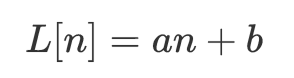
Fourier-transform for Time-Series: Detrending

Detrending your time-series might be a game-changer

Detrending a signal before computing its Fourier transform is a common practice, especially when dealing with time-series.

In this post, I want to show both mathematically and visually how detrending your signal affects its Fourier-transform.

All images by author.

This post is the fourth of my Fourier-transform for time-series series: I use very simple examples and a few mathematical formulas to explain various concepts of the Fourier transform. You don’t need to read them in the order below, I’d rather recommend going back and forth between each article.

Check out the previous posts here:

• Review how the convolution relate to the Fourier transform and how fast it is:

• Deepen your understanding of convolution using image examples:

• Understand how the Fourier-transform can be visualy understood using a vector-visual approach:

In this post, we are going to explore 2 kinds of detrends : we’ll call them ‘constant’ and ‘linear’ detrendings.

The end goal of this post is to make you understand what are constant and linear detrending, why we use them, and how they affects the Fourier-transform of the signal.

Quick review of the Fourier transform

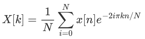
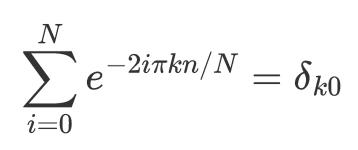
In this post, we’ll use the following definition of the Fourier-transform : for an input sequence x[n], for n=0 to N, the k-th coefficient of the Fourier-transform is the following complex number:

Constant detrending

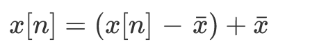
Let’s analyse the input signal. The sequence x[n] can be decomposed as follow: instead of considering x as a whole, let’s write it as a sum of 2 signals : a ‘constant part’ equal to the mean of the signal, and a ‘variability around the mean’ part giving the difference between the actual signal and its mean:

So for all sample n, we have:

First, let’s take the Fourier transform of the mean of x :

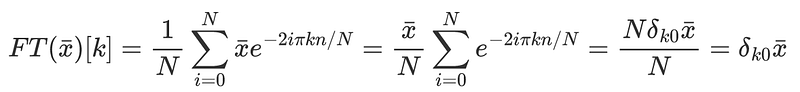
Which is a simple sequence with value the mean of x at sample k=0, and 0 everywhere else. Using the code from the previous post, we can easily understand why the following is true:

import numpy as np
import matplotlib.pyplot as plt

N = 10
ns = np.arange(N)

fig, axes = plt.subplots(1, N//2+1, figsize=(18,8), sharex=True, sharey=True)

for k in range(0, N//2+1):
    eiks = np.exp(-2*1J*np.pi*ns/N*k)
    pretty_ax(axes[k])
    plot_sum_vector(eiks, axes[k])
    axes[k].set_title(f'k={k}')
    axes[k].set_aspect('equal')
fig.suptitle(f'Complex plot of the $e^{{-2i\pi kn/N}}$ families')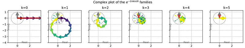

Now let’s take the Fourier tranform of x as we wrote it, with its 2 parts :

In other words, the Fourier transform of x is the sum of the Fourier transform of its variability around its mean, plus a sequence that is 0 everywhere except for k=0 where its equals the mean of x.

And that’s what constant detrending is : it just means to remove the mean of the signal before taking its Fourier-transform. In terms of Fourier coefficients, it corresponds to setting 0 to the k=0 coefficient.

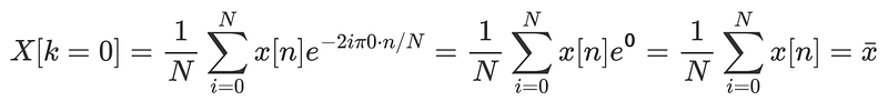
Another way to see this is the following: it can be shown easily that the coefficient for k=0 is always equal to the mean of the signal:

Linear detrending

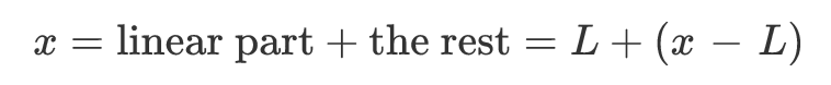
The approach is the same as before: write the input signal a sum of 2 parts: a “linear” part, and the rest of variability around this linear part:

where the linear part is typically computed from a least-square fit. Using indexes we can write the linear part as :

with b being the mean of the signal.

Now that we have written the decomposition of x, let’s take its Fourier-transform :

with the Fourier-transform of the linear part being, given the linearity property of the Fourier-transform:

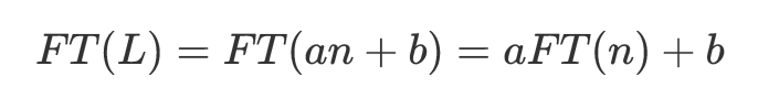
So linear detrending consists in removing the linear part of x before taking its Fourier-transform: it removes the term aFT(n)+b from the result, where a is a constant factor (corresponding to the slope of the linear fit), FT(n) is the Fourier transform of the linear sequence [0, 1, …], and b is the mean of the signal (hence the first Fourier coefficient will be 0, as in constant detrending).

Detrending in python

Let’s see how we can simply detrend a signal and take its Fourier transform in python. It is pretty straightforward using numpy and scipy.

Scipy proposes a detrend function in its signal package, with a type argument to specify if we want to constant-detrend or linear-detrend our signal.

In the example below, we create a signal of length 20 samples, that contains a linear part with leading coefficient 2, a bit of noise, an offset of 4, and a sinusoidal part.

import numpy as np
from scipy.signal import detrend
import matplotlib.pyplot as plt

N = 20
# create a sample signal, with linear, offset, noise and sinus parts
ys = np.arange(N) * 2 + 4 + np.random.randn(N) + 4*np.sin(2*np.pi*np.arange(N)/5)
# constant and linear detrend
ys_c = detrend(ys, type='constant')
ys_l = detrend(ys, type='linear')

fig, axes = plt.subplots(1, 2)

ax = axes[0]
ax.plot(ys, label='raw')
ax.plot(ys_c, label='constant-detrended')
ax.plot(ys_l, label='linear-detrended')
ax.legend()
ax.set_title('Input signal')

ax = axes[1]
# we use rfft since our input signals are real
ax.plot(np.abs(np.fft.rfft(ys)))
ax.plot(np.abs(np.fft.rfft(ys_c)))
ax.plot(np.abs(np.fft.rfft(ys_l)))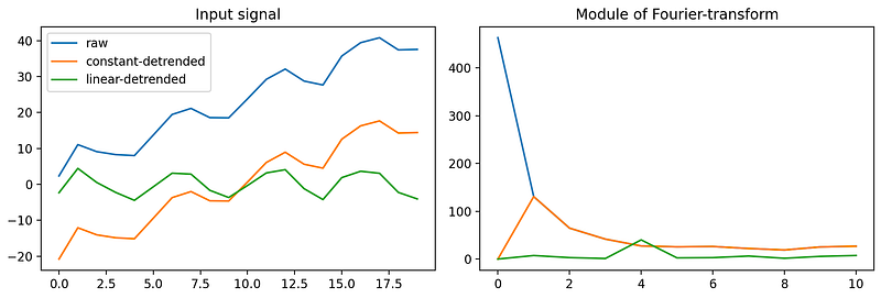
ax.set_title('Module of Fourier-transform')

Let’s review the plots.

On the left we have the raw input signal, as well as its constant-detrended and linear-detrended versions.

Constant detreding effectively removes the mean of the signal to center it around 0. Linear detrending not only removes the mean of the signal, but also its linear trend (aka “straight slope”). Visually, it is easier to spot the sinusoidal part on the linear-detrended signal than on the raw signal.

On the right are the modules of the Fourier-transform of each signal: If no detrend is applied, we get the blue module. Removing the mean using constant detrending effectively set the 0-th coefficient to 0, which most of the time make the plot easier to analyze. But the best part comes from linear-detrending: as you can see, the output Fourier coefficients shows well the sinus frequency in the ouput spectrum.

So imagine your are analyzing a time series and looking for seasonal patterns using the Fourier spectrum: it is way easier if your signal has been linear-detrended.

To go even further, the main advantage of linear-detrending is that it reduces spectral-leakage a lot. We’ll see in detail in another post what is spectral leakage and why we want to get rid of it.

About the Fourier-transform of a linear signal

We can easily plot the Fourier-transform of a linear signal Kn where K is the slope, for different values of K:

import numpy as np
import matplotlib.pyplot as plt

N = 10
ns = np.arange(N)
Ks = [-5, 2, 5]

fig, axes = plt.subplots(len(Ks), N//2+1, figsize=(18,8), sharex=True, sharey=True, gridspec_kw={'hspace':0, 'wspace':0})

for i, K in enumerate(Ks):
    xs = K*np.arange(N)
    for k in range(0, N//2+1):
        Zs = xs * np.exp(-2*1J*np.pi*ns/N*k) / N
        ax = axes[i, k]
        pretty_ax(ax)
        plot_sum_vector(Zs, ax)
        ax.set_aspect('equal')
        ax.set_xlabel(f'k={k}')
    axes[i, 0].set_ylabel(f'K={K}')
fig.tight_layout()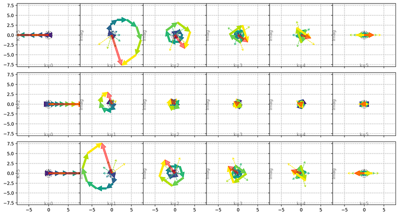

As you can see, for a given value of k, the Fourier-coefficients, represented by the red arrow, are always aligned, and equal up to a scale. So the removed part of the output spectrum is always that of the Fourier transform of the sequence [0, 1, …N], with a scaling factor given by the slope of the linear fit.

Wrapup

In this post, we saw what constant and linear detrending are: it simply consists of removing the mean or the linear fit of the input signal, respectively. This preprocessing step before computing the Fourier-transform helps make the output spectrum easier to interpret.

Removing the mean of the signal sets the 0-th coefficient to 0. The resulting plot is easier to inspect since, most of the time, the mean can be pretty big compared to the rest of the spectrum. So, the scale of the y-axis is easier to set if we remove that coefficient.

Removing the linear part, in addition to removing the mean, also removes the general trend in the signal, which is usually the dominating part of the raw signal and can hide the other components/seasonal behaviors that you’re really interested in.

If you liked this post and want to read more, please subscribe :) !

And make sure to check my other posts not Fourier-transform related:

• Finite difference method with numpy:

• Comparison between PCA, ICA and LDA algorithms:

• Compare PCA-whitening and ZCA-withening: