Forecasting the stock market using LSTM; will it rise tomorrow.

Using a machine learning model, this tutorial will predict a stock’s future value in real time with high accuracy on a stock exchange. To predict if the stock price will rise or fall tomorrow, we will use Google stock data as a time series. The data will be obtained from the Yfinance API.

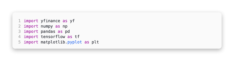
Prepare the project by importing the required libraries

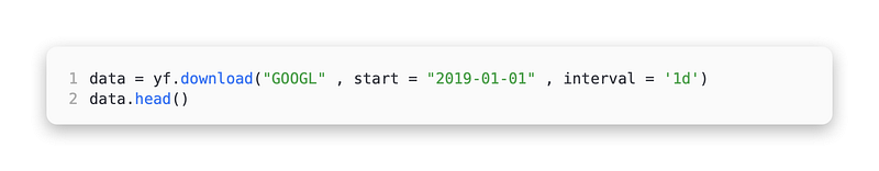
Using the Yfinance API, download Google stock data

In addition to checking the dataset details such as the data types of the features, we also need to check if there are any null values.

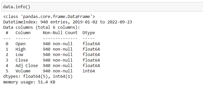
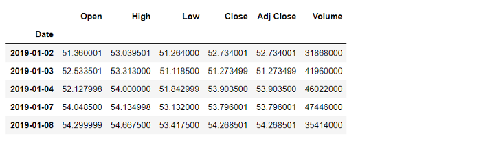
Six features are included in the dataset. Here are some of these features:

• Open. At the beginning of trading on a particular day, the stock’s price was
• High. During a trading day, the stock’s highest value
• Low. The lowest price at which a stock trades on a given day
• Close. During a trading day, this is the last price at which a stock traded
• Adj Close. Including any corporate actions, this is the stock’s closing price.
• Volume. During a particular period, the number of shares traded in a stock

On the New York Stock Exchange (NYSE), for instance, trading takes place from Monday through Friday from 9:30 a.m. through 4:00 p.m. ET. The opening price (open) is the price at which the stock starts trading, which is 9:30 a.m., and the closing price (close) is the price when the trading ends, which is 4:00 p.m. As an example, the New York Stock Exchange (NYSE) is open from 9:30 am to 4:00 pm Eastern time from Monday to Friday. In this case, the opening price (open) is what the stock is worth when it starts trading at 9:30 am and the closing price (close) is what it is worth when it ends trading at 4:00 pm.

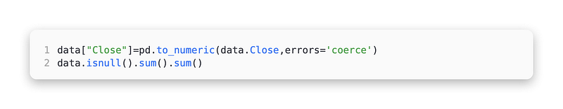
In the next step, we will check for non-numeric values in the ‘Close’ feature and change them to Nan. Check for non-numeric values in the dataset as well.

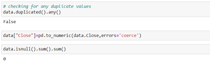
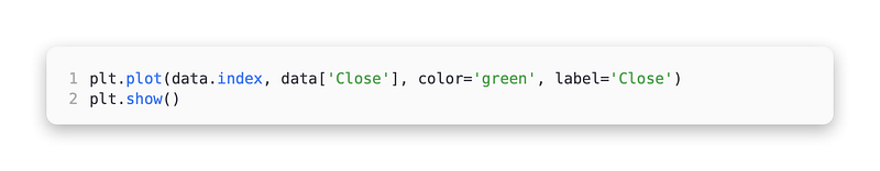
There are no Nan values associated with the ‘Close’ feature. In the next step, we will plot the close and check the stock’s growth based on the time.

Processing of data

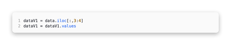
Due to the limited number of features we are going to use in this tutorial, a new dataframe will be created, dataV1, and only contain the Close feature.

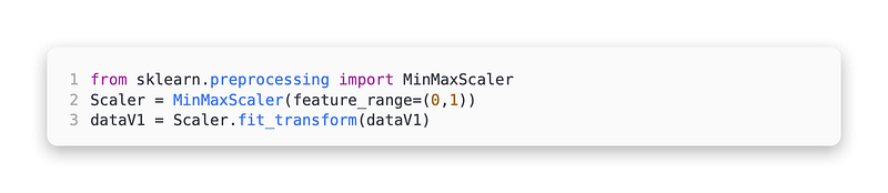
To normalize our data, import MinMaxScaler from sklearn library. It does this by transforming a feature by scaling it to a given range in this case just the ‘Close’ feature.

The feature length should be declared

Our data has to be divided into X and Y variables before we can build the model. To do so, we will write a function called Create_Features_and_Targets.

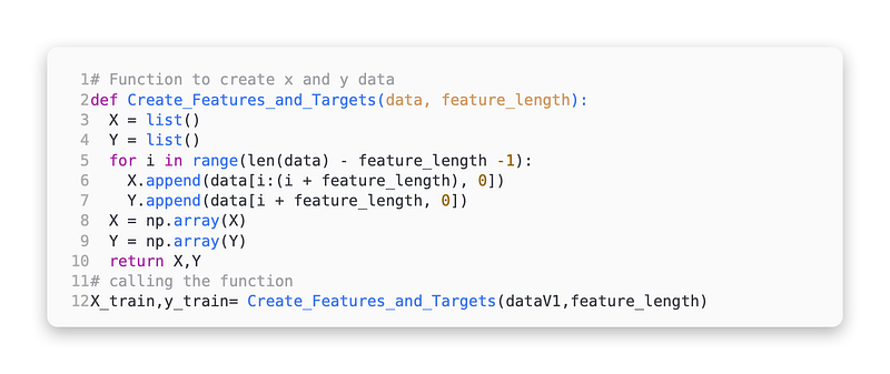
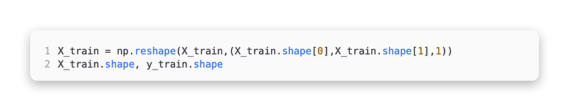
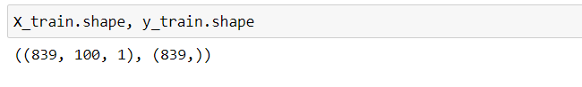
As LSTM takes 3 dimensional data as input, data should be made 3 dimensional.

Model creation

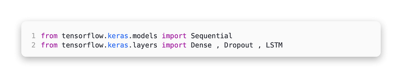
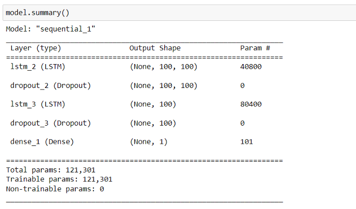
Create the model by importing the required libraries

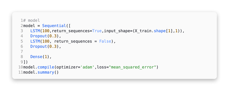
Adam will be used as an optimizer for the LSTM model we will create which consists of two LSTM layers, two dropout layers, and one dense layer.

How does LSTM work?

LSTMs are recurrent neural networks (RNNs). In simple terms, LSTMs work by allowing the network to remember the context of the model while forgetting the irrelevant information.

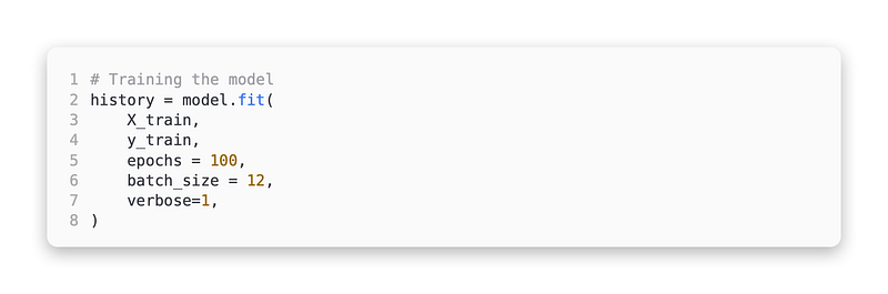
The data has already been prepared and the model has been developed. Using the model.fit function, we can now train the model. Our model will be trained using a batch_size of 12 under 100 epochs.

It’s time to test the model now that we have successfully trained it. For testing the model, the whole data set will be used, and the predicted data will be plotted against the actual data.

Predicting and testing

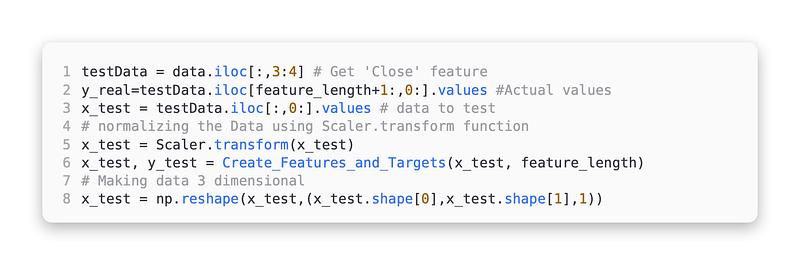
To run the tests, you will need to collect data from two datasets. The ‘Close’ feature should be used to create two variables, one for plotting real data, y_real, and one for making predictions, x_test. Our goal is to create the x_test variable by getting all the values from the ‘Close’ feature, scaling the data with Scaler.transform and transforming the shape to a 3D shape. From the ‘Close’ feature, we can get all values starting from the 101st value to create the y_real variable.

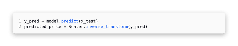
Making predictions

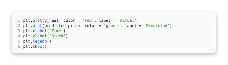
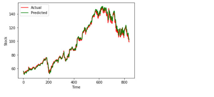
Now let’s plot the data after running the prediction test

Comparison of predicted and actual stock prices

Predictions in real time

Here’s a real-time prediction we can make. The objective of this exercise is to create a function that predicts the stock price on a given date.

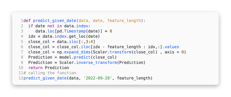
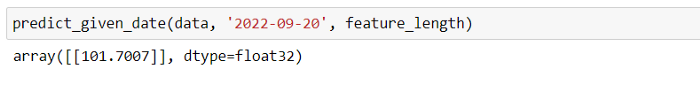
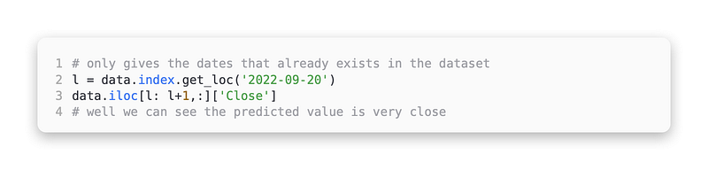
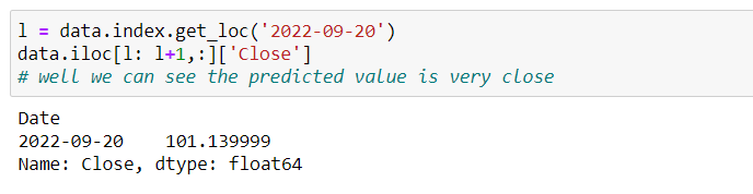
Taking a look at our model’s prediction for the given date of 2022–09–20, let’s see if it’s any closer to the actual price on that date. Here is the code that does just that. If the date provided already exists in the dataset, this gives the correct result.

The practical guide has come to an end. Despite the fact that we can make this better, I do not recommend using it for real-time trading at this time.

Thank you for taking the time to read this tutorial. I hope you enjoyed it. I appreciate your time.