Forecasting Stock Prices with Advanced Recurrent Neural Networks: A Comparative Analysis of LSTM, GRU, and Hybrid Models

In this article, we will explore the use of advanced recurrent neural network models — LSTM, GRU, and a hybrid of both — to predict Amazon’s stock prices based on historical data. Our findings suggest that these machine learning techniques hold significant potential for financial forecasting, demonstrating the capability to capture temporal dependencies in the data and model market dynamics effectively.

The LSTM, GRU, and hybrid models were trained on Amazon’s historical stock price data retrieved from Quandl and were used to predict future prices. Each model was evaluated based on its ability to closely match the actual stock prices. This study contributes to the ongoing discourse on AI’s increasing role in financial services, particularly in the stocks sector.

Future work could explore tuning these models further or investigate other machine-learning techniques to enhance prediction accuracy. Additionally, incorporating other features like market indicators or global economic factors could also provide a more comprehensive prediction model. While the results are promising, it’s important to remember that stock price prediction is inherently uncertain and should be one of many tools used in financial decision-making.

import numpy as np
import matplotlib.pyplot as plt
plt.style.use('fivethirtyeight')
import pandas as pd
from sklearn.preprocessing import MinMaxScaler
from keras.models import Sequential
from keras.layers import Dense, LSTM, Dropout, GRU, Bidirectional
from keras.optimizers import SGD
import math
from sklearn.metrics import mean_squared_error

Data processing, visualization, and modeling tasks are performed using this code. It begins by importing several libraries and modules that are commonly used in these tasks. First, the ‘numpy’ library is imported with the alias ‘np’. Mathematical functions and tools for arrays and matrices are provided by Numpy. It is widely used for numerical computations in Python. The next step is to import the ‘matplotlib.pyplot’ module with the alias ‘plt’. Plots and charts are created using this module. It provides a wide range of functions to generate different types of plots and customize their appearance. The plots are also styled as ‘fivethirtyeight’.

Data visualization in this style is known for its clean and modern appearance. By using this style, the resulting plots will have a consistent aesthetic. Additionally, the ‘pandas’ library is imported as ‘pd’. The Pandas library is a powerful tool for manipulating and analyzing data. It provides data structures, such as DataFrames, and a wide range of functions for handling and processing data.

For example, the MinMaxScaler class is imported from the ‘sklearn.preprocessing’ module. Scaling data between 0 and 1 is accomplished using this class. It is commonly used in machine learning tasks to normalize the data and bring it into a suitable range for modeling. Several classes are imported from the keras library, which is a popular deep learning library. In neural network models, the ‘Sequential’ class represents a linear stack of layers. In a neural network model, the ‘Dense’, ‘LSTM’, ‘Dropout’, ‘GRU’, and ‘Bidirectional’ classes define different types of layers. These classes are building blocks for constructing deep learning models. The ‘SGD’ optimizer is imported from the keras.optimizers module.

Stochastic Gradient Descent is a popular optimization algorithm used to train neural networks. It adjusts the model’s parameters iteratively to minimize the loss function. The ‘math’ module provides mathematical functions and constants. It can be used for various mathematical operations and calculations. Furthermore, the ‘mean_squared_error’ function from the ‘sklearn.metrics’ module is imported. It calculates the mean squared error between predicted and actual values. It is a common metric used to evaluate the performance of regression models.

To summarize, this code sets up the necessary environment for data processing, visualization, and modeling tasks. It is possible to manipulate data, create visualizations, and build deep learning models using these tools.

import pandas as pd
import quandl
import datetime
start = datetime.datetime(2006,1,1)
end = datetime.date.today()
amz = quandl.get("WIKI/AMZN", start_date=start, end_date=end)

This code performs several tasks related to retrieving historical stock price data for Amazon (AMZN) using the Quandl platform. The pandas library is imported and given the alias pd. In Python, Pandas is a powerful library for manipulating and analyzing data. It provides data structures and functions that make it easier to work with structured data, such as tables or spreadsheets.

After that, the code imports the Quandl module, which provides access to a variety of financial, economic, and alternative datasets. Quandl is a popular data provider that offers a comprehensive collection of historical data. The ‘datetime’ module is also included. Python provides classes and functions for working with dates and times. It enables operations such as creating, formatting, and manipulating dates and times. Using the ‘datetime.datetime’ class, a ‘start’ variable is defined. Historical stock price data are retrieved starting from this variable. In this case, the start date is set to January 1, 2006. An ‘end’ variable is also created using ‘datetime.date.today()’. The current date is used as the end date for retrieving data.

By using the ‘datetime.date.today()’ function, the code automatically sets the end date to the present day. To retrieve Amazon stock price data, the code uses the ‘quandl.get’ function. This specifies the dataset to be retrieved as “WIKI/AMZN”, indicating Amazon’s stock price data from the WIKI database on Quandl. A ‘start’ and ‘end’ date is used as parameters to determine the time range for which the data will be retrieved. A variable named ‘amz’ is used to store the retrieved data, which can be analyzed, processed, or visualized using the ‘pandas’ library’s functionalities. This code creates the necessary environment to retrieve Amazon historical stock price data.

In this program, the necessary libraries are imported, the start and end dates for data retrieval are defined, and the Quandl platform is used to fetch the desired data set. Resulting data is stored in a variable for further analysis.

# Some functions to help out with
def plot_predictions(test,predicted):
    plt.plot(test, color='red',label='Real Amazon Stock Price')
    plt.plot(predicted, color='blue',label='Predicted Amazon Stock Price')
    plt.title('Amazon Stock Price Prediction')
    plt.xlabel('Time')
    plt.ylabel('Amazon Stock Price')
    plt.legend()
    plt.show()

def return_rmse(test,predicted):
    rmse = math.sqrt(mean_squared_error(test, predicted))
    print("The root mean squared error is {}.".format(rmse))

In the given code, two functions are defined: plot_predictions and return_rmse. These functions are designed to assist with data visualization and error evaluation in the context of stock price prediction. Specifically, plot_predictions takes two parameters, test and predicted. With the help of the ‘matplotlib.pyplot’ library, it creates a plot with two lines: one representing the real Amazon stock prices and the other representing predicted Amazon stock prices. A title, labels for the axes, and a legend are also set by the function. Finally, it displays the plot on the screen. The return_rmse function calculates the root mean square error (RMSE) between the test value and the predicted value.

A regression model’s RMSE is a commonly used metric to measure its accuracy. The average difference between the predicted and actual values is quantified. As a formatted string, the function prints the RMSE derived from the functions ‘math.sqrt’ and ‘mean_squared_error’. Overall, these functions provide a convenient way to visualize predicted stock prices compared to actual prices and to evaluate the performance of a prediction model using the RMSE metric.

dataset = pd.read_csv('AMZN_2006-01-01_to_2018-01-01.csv', index_col='Date', parse_dates=['Date'])
dataset.head()

It reads a CSV file named ‘AMZN_2006–01–01_to_2018–01–01.csv’ and assigns its contents to a variable called ‘dataset’. The CSV file is expected to contain stock price data for Amazon (AMZN) within a specific time range. This data can be read using the ‘pd.read_csv’ function of the pandas library. Data is loaded into a pandas DataFrame using the file path as a parameter. As the ‘index_col’ parameter is set to ‘Date’, the CSV file’s ‘Date’ column will be used as the DataFrame’s index. The ‘parse_dates’ parameter is set to [‘Date’], which instructs pandas to interpret the ‘Date’ column as a datetime data type. The ‘dataset.head()’ function is then called.

In this function, the first few rows of the DataFrame are displayed, providing a preview of the data. By default, it shows the first five rows. This code reads a CSV file containing Amazon stock price data, assigns it to a DataFrame called ‘dataset’, and displays the first few rows. As a result, the data can be explored and the structure of the data can be understood.

training_set = dataset[:'2016'].iloc[:,1:2].values
test_set = dataset['2017':].iloc[:,1:2].values

This code divides the ‘dataset’ into two sets: a training set and a test set, based on specific date ranges. The training set contains data up to 2016. Slicing the dataset by ‘2016’ includes all rows from the beginning up to (but not including) the year 2016 in the selection. The `.iloc[:,1:2]` part specifies that only the second column (index 1) of the dataset is used for training. The `.values` at the end returns the selected data as a NumPy array. Meanwhile, the test set contains data from 2017 onwards. As the slicing notation indicates, the dataset contains all rows beginning in 2017 until the end. The `.iloc[:,1:2]` part ensures that only the second column of the dataset is included. The `.values` at the end returns the selected data as a NumPy array.

To summarize, this code divides the dataset into a training and test set. The training set contains data up to 2016, while the test set contains data up to 2017. As NumPy arrays, both sets consist of values from the second column of the original dataset.

#We have chosen 'High' attribute for prices. Let's see what it looks like
dataset["High"][:'2016'].plot(figsize=(16,4),legend=True)
dataset["High"]['2017':].plot(figsize=(16,4),legend=True)
plt.legend(['Training set (Before 2017)','Test set (2017 and beyond)'])
plt.title('AMAZON stock price')
plt.show()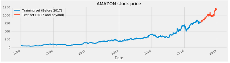

Based on the ‘High’ attribute, this code visualizes the historical stock prices of Amazon (AMZN). The plot is divided into two parts to represent the training set and the test set, corresponding to different time periods.

The first part of the code, `dataset[“High”][:’2016'].plot(figsize=(16,4),legend=True)`, plots the ‘High’ attribute of the ‘dataset’ variable for the data up until the year 2016. The plot is created using the pandas library’s ‘plot’ function. The ‘figsize’ parameter sets the size of the figure, and ‘legend=True’ displays the legend in the plot.

The second part of the code, `dataset[“High”][‘2017’:].plot(figsize=(16,4),legend=True)`, plots the ‘High’ attribute of the ‘dataset’ variable for the data from the year 2017 onwards. This part uses the same ‘plot’ function but with a different slicing notation to select the data from the year 2017 onwards. A legend is added to the plot using the ‘plot.legend’ function. It specifies the labels for the legend as ‘Training set (Before 2017)’ and ‘Test set (2017 and beyond)’ to distinguish the two parts of the plot. Finally, it specifies that the plot represents the Amazon stock price by using the ‘plt.title’ function. The plot is then displayed using the ‘plt.show’ function. This code visualizes historical Amazon stock prices based on the ‘High’ attribute. Using the legend, the plot is divided into a training set (data before 2017) and a test set (data after 2017). Over time, the plot shows the stock price trends.

# Scaling the training set
sc = MinMaxScaler(feature_range=(0,1))
training_set_scaled = sc.fit_transform(training_set)

This code performs data scaling on the training set using the MinMaxScaler. It is part of the sklearn.preprocessing module. This scaling technique transforms the data into a specific range, typically between 0 and 1. Scaling the data is beneficial for many machine learning algorithms as it helps in normalizing the data and bringing it into a consistent range. It is done using the ‘fit_transform’ method of the ‘MinMaxScaler’ class. To scale the data, it computes the minimum and maximum values of the training set. The scaled data is then assigned to the ‘training_set_scaled’ variable. The code uses the MinMaxScaler to normalize the data and ensure that it falls within a specified range. Scaled data is stored in the training_set_scaled variable and can be used for further analysis.

LSTMs store long-term memory state, so we create a data structure with 60 timesteps and 1 output. We have 60 elements of previous training sets for each element of training set

X_train = []
y_train = []
for i in range(60,2768):
    X_train.append(training_set_scaled[i-60:i,0])
    y_train.append(training_set_scaled[i,0])
X_train, y_train = np.array(X_train), np.array(y_train)

By creating input sequences and target values, this code prepares the training data for a machine learning model. To store the input sequences and target values, the code initializes two empty lists called ‘X_train’ and ‘y_train’. A for loop is used to iterate over the range of indices from 60 to 2768. This range represents the indices of the training set data. During each iteration, 60 elements from the ‘training_set_scaled’ list are appended to the ‘X_train’ list. In the first column (index 0) of the ‘training_set_scaled’, the ‘[i-60:i,0]’ notation selects values from index ‘i-60’ to index ‘i’ to produce the sequence.

Moreover, the element at index ‘i’ from the ‘training_set_scaled’ list is appended to the ‘y_train’ list as well. As a result of the input sequence, this element represents the target value. Using ‘np.array’ function, the ‘X_train’ and ‘y_train’ lists are converted into NumPy arrays, which produce final training data consisting of input sequences (‘X_train’) and target values (‘y_train’). Based on the scaled training set data, this code generates input sequences and target values. Input sequences consist of 60 consecutive elements, while target values are single values. In a machine learning model, these sequences and target values are stored as NumPy arrays.

# The LSTM architecture
regressor = Sequential()
# First LSTM layer with Dropout regularisation
regressor.add(LSTM(units=50, return_sequences=True, input_shape=(X_train.shape[1],1)))
regressor.add(Dropout(0.2))
# Second LSTM layer
regressor.add(LSTM(units=50, return_sequences=True))
regressor.add(Dropout(0.2))
# Third LSTM layer
regressor.add(LSTM(units=50, return_sequences=True))
regressor.add(Dropout(0.2))
# Fourth LSTM layer
regressor.add(LSTM(units=50))
regressor.add(Dropout(0.2))
# The output layer
regressor.add(Dense(units=1))

# Compiling the RNN
regressor.compile(optimizer='rmsprop',loss='mean_squared_error')
# Fitting to the training set
regressor.fit(X_train,y_train,epochs=5,batch_size=32)

This code defines and trains a specific type of recurrent neural network (RNN) architecture called Long Short-Term Memory (LSTM) for a regression task. It begins by creating a sequential model called ‘regressor’ using the Keras Sequential class. This model will serve as the container for the LSTM layers and other components. The code then adds several LSTM layers. LSTM layers are added using the ‘regressor.add’ function. Each LSTM layer is specified by the ‘units’ parameter. For all LSTM layers except the last, the ‘return_sequences’ parameter is set to ‘True’, indicating that each layer should return sequences rather than just the final result. With a dropout rate of 0.2, the ‘Dropout’ layer is added after each LSTM layer. Dropout is a regularization technique that helps prevent overfitting in neural networks.

A dense layer with a single unit is added after the LSTM layers. This layer is responsible for producing the regression output. After that, the RNN model is compiled using the ‘regressor.compile’ function. In this example, the ‘optimizer’ parameter is set to ‘rmsprop’, which is an optimization algorithm commonly used for training RNNs. The ‘loss’ parameter is set to ‘mean_squared_error’, indicating that the mean squared error is used as the loss function to measure the model’s performance. Finally, the model is fitted using the ‘regressor.fit’ function.

Preprocessed training data (‘X_train’ and ‘Y_train’) are input along with parameters such as epochs (5) and batch size (32). During the training process, the model iteratively adjusts its weights and biases to minimize the mean squared error loss between the predicted and actual values. To summarize, this code defines and trains an LSTM-based RNN model. It consists of multiple LSTM layers with dropout regularization, an output layer, and is trained using the mean squared error loss function.

Here is how to prepare the test set in the same way as the training set.The following has been done so forst 60 portions of the test set have 60 previous values, which are impossible to obtain unless we process all ‘High’ attribute data.

dataset_total = pd.concat((dataset["High"][:'2016'],dataset["High"]['2017':]),axis=0)
inputs = dataset_total[len(dataset_total)-len(test_set) - 60:].values
inputs = inputs.reshape(-1,1)
inputs  = sc.transform(inputs)

This code preprocesses the input data for making predictions by combining the ‘High’ attribute values from two subsets of the ‘dataset’ and scaling them. The ‘dataset_total’ variable is created by concatenating two subsets of the ‘High’ attribute. The first subset contains data until 2016, and the second subset contains data from 2017 onwards. Concatenation is performed using the ‘pd.concat’ function from the pandas library, with the ‘axis=0’ parameter specifying the concatenation along the vertical axis. Inputs is defined by extracting a portion of the dataset_total array. This function selects a range of values starting from a position calculated as the length of ‘dataset_total’ minus the length of ‘test_set’ minus 60. In this way, the inputs are aligned with the test set’s time period, and preceding values are included for making predictions.

The input array is reshaped using the ‘reshape’ method, where ‘-1’ indicates that the dimension is inferred based on the input array’s length. The reshaping is done to ensure that the ‘inputs’ array has a single feature dimension, as expected by the subsequent operations. Finally, the ‘sc.transform’ function is used to scale the ‘inputs’ array. ‘sc’ represents the MinMaxScaler object that scaled the training set previously. Inputs are scaled according to the same scaling as the training set by calling ‘transform’ on ‘sc’ and passing the input array as a parameter.

In summary, this code combines subsets of the ‘High’ attribute from the ‘dataset’, extracts a portion of the combined data to form the ‘inputs’ array, reshapes the ‘inputs’ array, and scales it using the same scaling transformation as applied to the training set. During these steps, the input data is prepared for further processing and prediction.

# Preparing X_test and predicting the prices
X_test = []
for i in range(60,311):
    X_test.append(inputs[i-60:i,0])
X_test = np.array(X_test)
X_test = np.reshape(X_test, (X_test.shape[0],X_test.shape[1],1))
predicted_stock_price = regressor.predict(X_test)
predicted_stock_price = sc.inverse_transform(predicted_stock_price)

This code prepares the input data for testing and uses a trained model to predict stock prices. Using a for loop, the code iterates over a range of indices from 60 to 311. This range represents the indices of the ‘inputs’ array, which was previously prepared and scaled. Each iteration adds 60 consecutive elements from the inputs array to the ‘X_test’ array. This sequence is obtained using the slicing notation ‘[i-60:i,0]’, which selects the values from ‘i-60’ to ‘i’ in the first column (index 0) of the inputs array. After the loop completes, the ‘X_test’ list is converted into a NumPy array using the ‘np.array’ function. The array is then reshaped to match the input shape expected by the trained model. Reshaping is performed using ‘np.reshape’, with the desired shape specified as (X_test.shape[0], X_test.shape[1], 1).

This ensures that the dimensions of the ‘X_test’ array align with the number of samples, the length of each sequence, and the number of features (in this case, 1). Based on the ‘X_test’ input, the trained model, ‘regressor’, predicts stock prices. The ‘predict’ method is called on ‘regressor’ with ‘X_test’ as the input, resulting in an array of predicted stock prices. The ‘inverse_transform’ method is applied to the predicted stock price array to obtain the actual stock price value. This method uses the scaling transformation applied earlier to revert the scaled values back to their original scale. To summarize, this code creates sequences based on the scaled ‘inputs’ array. The ‘X_test’ array is reshaped to match the input shape expected by the model. A trained model is then used to predict stock prices for the prepared ‘X_test’ input. The predicted stock prices are then transformed back to their original scale.

# Visualizing the results for LSTM
plot_predictions(test_set,predicted_stock_price)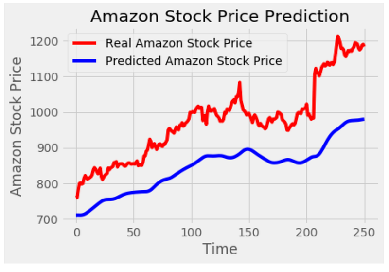

This code generates a visualization of the predicted stock prices from an LSTM model and compares them to the actual stock prices. This code calls the function ‘plot_predictions’ and passes two parameters: ‘test_set’ and ‘predicted_stock_price’. The ‘test_set’ represents the actual stock prices, while ‘predicted_stock_price’ contains the predicted stock prices from the LSTM model. A plot is created using the ‘matplotlib.pyplot’ library. To represent actual stock prices, it plots the ‘test_set’ as a red line. Additionally, it plots the ‘predicted_stock_price’ as a blue line to represent the predicted stock prices. This plot is titled ‘Amazon Stock Price Prediction’. With the ‘plt.xlabel’ function, the x-axis is labeled as ‘Time’, and the y-axis is labeled as ‘Amazon Stock Price’. Using the ‘plt.legend’ function, a legend is added to the plot to distinguish between actual and predicted stock prices. With the ‘plt.show’ function, the plot is displayed on the screen. The code visualizes the predicted stock prices from the LSTM model and compares them to the actual stock prices. Plotting the stock prices helps visualize the model’s accuracy and understand the trend and pattern.

regressorGRU = Sequential()
# First GRU layer with Dropout regularisation
regressorGRU.add(GRU(units=50, return_sequences=True, input_shape=(X_train.shape[1],1), activation='tanh'))
regressorGRU.add(Dropout(0.2))
# Second GRU layer
regressorGRU.add(GRU(units=50, return_sequences=True, input_shape=(X_train.shape[1],1), activation='tanh'))
regressorGRU.add(Dropout(0.2))
# Third GRU layer
regressorGRU.add(GRU(units=50, return_sequences=True, input_shape=(X_train.shape[1],1), activation='tanh'))
regressorGRU.add(Dropout(0.2))
# Fourth GRU layer
regressorGRU.add(GRU(units=50, activation='tanh'))
regressorGRU.add(Dropout(0.2))
# The output layer
regressorGRU.add(Dense(units=1))
# Compiling the RNN
regressorGRU.compile(optimizer=SGD(lr=0.01, decay=1e-7, momentum=0.9, nesterov=False),loss='mean_squared_error')
# Fitting to the training set
regressorGRU.fit(X_train,y_train,epochs=5,batch_size=150)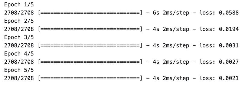

This code defines and trains a specific type of recurrent neural network (RNN) architecture called Gated Recurrent Unit (GRU) for a regression task. First, an empty sequential model is created using Keras’ Sequential class. This model will serve as the container for the GRU layers and other components. The code adds several GRU layers next. The ‘regressorGRU.add’ function is used to add each GRU layer. In each GRU layer, the ‘units’ parameter specifies the number of memory cells or units. GRU layers except the last one have the ‘return_sequences’ parameter set to ‘True’, indicating that each layer should return sequences instead of just the final result. ‘input_shape’ specifies the shape of the input data, which is derived from ‘X_train’.

The ‘activation’ parameter is set to ‘tanh’, which is the activation function used in the GRU layers. An output layer is added using ‘regressorGRU.add’. A dense layer with a single unit makes up the layer. This layer is responsible for producing the regression output. Next, the RNN model is compiled using the ‘regressorGRU.compile’ function. SGD stands for Stochastic Gradient Descent, and specific parameters are provided to configure the optimizer, such as the learning rate (‘lr’), decay, momentum, and Nesterov momentum.

The ‘loss’ parameter is set to ‘mean_squared_error’, indicating that the mean squared error is used as the loss function to measure the model’s performance. Finally, the model is trained using ‘regressorGRU.fit’. Input parameters include preprocessed training data (‘X_train’ and ‘y_train’), as well as the number of epochs (5) and batch size (150). During the training process, the model iteratively adjusts its weights and biases to minimize the mean squared error loss between the predicted and actual values. To summarize, this code defines and trains a GRU-based regression model. Using the mean squared error loss function, the model consists of multiple GRU layers with dropout regularization.

# Preparing X_test and predicting the prices
X_test = []
for i in range(60,311):
    X_test.append(inputs[i-60:i,0])
X_test = np.array(X_test)
X_test = np.reshape(X_test, (X_test.shape[0],X_test.shape[1],1))
GRU_predicted_stock_price = regressorGRU.predict(X_test)
GRU_predicted_stock_price = sc.inverse_transform(GRU_predicted_stock_price)

This code prepares the input data for testing and uses a trained GRU model to predict stock prices. First, an empty list called ‘X_test’ is created to store the input sequences. In a for loop, the code iterates over the indices 60 to 311. This range represents the indices of the ‘inputs’ array, which was previously prepared and scaled. During each iteration, 60 consecutive elements from the ‘inputs’ array are appended to the ‘X_test’ array. Using the slicing notation ‘[i-60:i,0]’, the sequence is obtained by selecting a range of values from index ‘i-60’ to ‘i’ in the first column (index 0). After the loop completes, the ‘X_test’ list is converted into a NumPy array using the ‘np.array’ function. After the array is converted, it is reshaped to match the input shape predicted by the trained GRU model. By using the ‘np.reshape’ function, the desired shape is specified as (X_test.shape[0], X_test.shape[1], 1). As a result, the dimensions of the ‘X_test’ array are aligned with the number of samples, the length of each sequence, and the number of features (in this case, 1).

On the basis of the input ‘X_test’, the trained GRU model, ‘regressorGRU’, predicts stock prices. The ‘predict’ method is called on ‘regressorGRU’ with ‘X_test’ as the input, resulting in an array of predicted stock prices. The ‘inverse_transform’ method is used to get the actual stock prices. This method uses the scaling transformation applied earlier to revert the scaled values back to their original scale. To summarize, this code prepares the input data for testing by creating sequences from the scaled inputs array. The GRU model reshapes the ‘X_test’ array to match the expected input shape. Using the trained GRU model, the stock prices for the prepared ‘X_test’ input are predicted. The predicted stock prices are then transformed back to their original scale.

# Visualizing the results for GRU
plot_predictions(test_set,GRU_predicted_stock_price)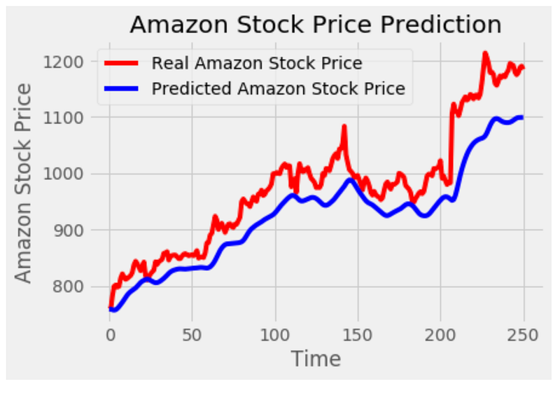

This code generates a visualization of the predicted stock prices from a GRU model and compares them to the actual stock prices. The function ‘plot_predictions’ is called with two parameters: ‘test_set’ and ‘GRU_predicted_stock_price’. The ‘test_set’ represents the actual stock prices, while ‘GRU_predicted_stock_price’ contains the predicted stock prices from the GRU model. A plot is created using the ‘matplotlib.pyplot’ library. To represent the actual stock prices, the ‘test_set’ is plotted as a red line. Additionally, it plots the ‘GRU_predicted_stock_price’ as a blue line to represent the predicted stock prices. This plot is titled ‘Amazon Stock Price Prediction’. Using the ‘plt.xlabel’ function, the x-axis is labeled ‘Time’, and the y-axis is labeled ‘Amazon Stock Price’. The ‘plt.legend’ function adds a legend to the plot to differentiate between the actual and predicted stock prices.

Finally, the plot is displayed on the screen using the ‘plt.show’ function.

Overall, this code visualizes the stock price predicted by a GRU model compared to the actual price. This plot helps visualize the accuracy of the model’s predictions and understand the stock price trend and pattern.

# The LSTM architecture
regressorLG = Sequential()
# First LSTM layer with Dropout regularisation
regressorLG.add(LSTM(units=50, return_sequences=True, input_shape=(X_train.shape[1],1)))
regressorLG.add(Dropout(0.2))
regressorLG.add(GRU(units=50, activation='tanh'))
regressorLG.add(Dropout(0.2))
# The output layer
regressorLG.add(Dense(units=1))
# Compiling the RNN
regressorLG.compile(optimizer=SGD(lr=0.01, decay=1e-7, momentum=0.9, nesterov=False),loss='mean_squared_error')
# Fitting to the training set
regressorLG.fit(X_train,y_train,epochs=5,batch_size=150)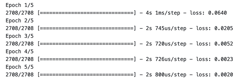

This code defines and trains a specific type of recurrent neural network (RNN) architecture that combines LSTM and GRU layers for a regression task. It begins by creating a sequential model called ‘regressorLG’ using Keras’ Sequential class. This model will serve as the container for the LSTM and GRU layers and other components. This next step adds an LSTM layer to the model using the regressorLG.add function. In the LSTM layer, the ‘units’ parameter specifies how many memory cells or units there are. A layer should return sequences if the ‘return_sequences’ parameter is set to ‘True’. ‘input_shape’ specifies the shape of the input data based on the shape of ‘X_train’. A dropout layer with a dropout rate of 0.2 follows this LSTM layer. Dropout is a regularization technique that helps prevent overfitting in neural networks. The GRU layer is added after the LSTM layer. In the GRU layer, the ‘units’ parameter specifies the number of memory cells or units. In the GRU layer, the ‘activation’ parameter is set to ‘tanh’. Another dropout layer is added after the GRU layer with a dropout rate of 0.2.

Finally, an output layer is added using ‘regressorLG.add’. There is a dense layer with a single unit in it. This layer is responsible for producing the regression output. The next step is to compile the RNN model using the ‘regressorLG.compile’ function. ‘Optimizer’ parameter is set to ‘SGD’, which stands for stochastic gradient descent, and specific parameters are provided to configure the optimizer, such as learning rate (‘lr’), decay, momentum, and Nesterov momentum. The ‘loss’ parameter is set to ‘mean_squared_error’, indicating that the mean squared error is used as the loss function to measure the model’s performance. The model is then trained using the ‘regressorLG.fit’ function.

In addition to the preprocessed training data (‘X_train’ and ‘Y_train’), it takes additional parameters such as the number of epochs (5) and batch size (150). During the training process, the model iteratively adjusts its weights and biases to minimize the mean squared error loss between the predicted and actual values. To summarize, this code defines and trains a regression model using LSTMs and GRUs. A model architecture consists of an LSTM layer, a dropout layer, a GRU layer, and another dropout layer. Using provided training data, the model is compiled with a specific optimizer and loss function.

# Preparing X_test and predicting the prices
X_test = []
for i in range(60,311):
    X_test.append(inputs[i-60:i,0])
X_test = np.array(X_test)
X_test = np.reshape(X_test, (X_test.shape[0],X_test.shape[1],1))
LG_predicted_stock_price = regressorLG.predict(X_test)
LG_predicted_stock_price = sc.inverse_transform(LG_predicted_stock_price)

This code prepares the input data for testing and uses a trained LSTM-GRU hybrid model to predict stock prices. The first step is to create an empty list called ‘X_test’ to store the input sequences. The loop iterates over 60 to 311 indices. This range represents the indices of the ‘inputs’ array, which was previously prepared and scaled. Each iteration adds 60 consecutive elements from the ‘inputs’ array to the ‘X_test’ array. It is obtained using the slicing notation ‘[i-60:i,0]’, which selects a range of values from index ‘i-60’ to ‘i’ in the first column (index 0) of the inputs array. These sequences serve as input data for making predictions. After the loop completes, the ‘X_test’ list is converted into a NumPy array using the ‘np.array’ function. Next, the NumPy array is reshaped to match the input shape of the trained LSTM-GRU model. Using the np.reshape function, the desired shape is specified as (X_test.shape[0], X_test.shape[1], 1). This ensures that the dimensions of the ‘X_test’ array are aligned with the number of samples, the length of each sequence, and the number of features (in this case, 1).

The trained LSTM-GRU model, ‘regressorLG’, is then used to predict the stock prices based on the prepared ‘X_test’ input. The ‘predict’ method is called on ‘regressorLG’ with ‘X_test’ as the input, resulting in an array of predicted stock prices. The inverse_transform method is used to obtain the actual stock price values from the predicted values. This method uses the scaling transformation applied earlier to revert the scaled values back to their original scale. Basically, this code prepares the input data for testing by creating sequences from the scaled input array. In order to match the input shape expected by the LSTM-GRU model, it reshapes the array ‘X_test’. In the next step, the trained LSTM-GRU model is used to predict the stock prices for the input ‘X_test’. The predicted stock prices are then transformed back to their original scale.

# Visualizing the results for GRU
plot_predictions(test_set,LG_predicted_stock_price)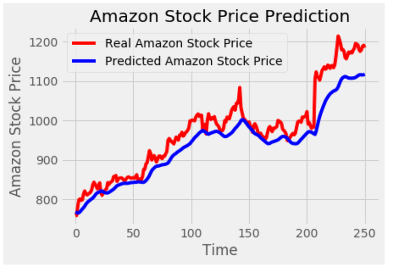

This code generates a visualization of the predicted stock prices from a LSTM-GRU hybrid model and compares them to the actual stock prices. The function plot_predictions takes two parameters: ‘test_set’ and ‘LG_predicted_stock_price’. The ‘test_set’ represents the actual stock prices, while ‘LG_predicted_stock_price’ contains the predicted stock prices from the LSTM-GRU model. Plots are created using the ‘matplotlib.pyplot’ library. ‘test_set’ is plotted as a red line to represent actual stock prices. Additionally, it plots the ‘LG_predicted_stock_price’ as a blue line to represent the predicted stock prices. The plot is titled ‘Amazon Stock Price Prediction’.

A ‘plt.xlabel’ function labels the x-axis as ‘Time’, and a ‘plt.ylabel’ function labels the y-axis as ‘Amazon Stock Price’. To distinguish between the actual and predicted stock prices, the ‘plt.legend’ function adds a legend to the plot. In summary, this code visualizes the predicted stock prices from a LSTM-GRU hybrid model and compares them to the actual stock prices. The plot is then displayed on the screen using the ‘plt.show’ function. In addition to illustrating the accuracy of the model’s predictions, the plot helps to understand the trend and pattern of stock price movements.

amz["High"][:'2017'].plot(figsize=(16,4),legend=True)
amz["High"]['2018':].plot(figsize=(16,4),legend=True)
plt.legend(['Training set (Before 2018)','Test set (2018 and beyond)'])
plt.title('AMAZON stock price')
plt.show()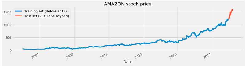

This code generates a plot to visualize the historical stock prices of Amazon, specifically the “High” attribute. The first line plots the “High” attribute of the ‘amz’ DataFrame, limiting the data to 2017. In the ‘[:’2017']’ slicing notation, rows from the beginning of the DataFrame up to 2017 are selected. The ‘plot’ function is called with additional parameters, such as ‘figsize=(16,4)’ to set the size of the plot, and ‘legend=True’ to display a legend. Line 2 plots the ‘High’ attribute of the ‘amz’ DataFrame. The slicing notation “[‘2018’:]” selects the rows from the year 2018 onward. It adds a legend with labels specifying the training and test sets. The ‘plt.title’ function sets the title of the plot as “AMAZON stock price”. Finally, the ‘plt.show’ function displays the plot on the screen. This code generates a plot that visualizes Amazon stock prices over time. Two lines represent the “High” attribute: one line for the training set up until 2017, and another line for the test set starting in 2018. A legend, a title, and a plot are displayed on screen.

# Scaling the training set
sc = MinMaxScaler(feature_range=(0,1))
training_set_scaled = sc.fit_transform(training_set)

This code performs scaling on the training set data to normalize the values within a specific range. It starts by creating an instance of the MinMaxScaler class. In feature scaling, this scaler transforms the data to a specified range. In this case, the feature range is set to (0, 1), meaning the scaled values will be between 0 and 1. ‘fit_transform’ is called on the scaler object with ‘training_set’ as the input. This method fits the scaler to the training set data and applies the scaling transformation to it. Scaled data is stored in the variable ‘training_set_scaled’. It contains the same data as the original training set, but with scaled values that fall within the specified feature range. To summarize, the code uses the MinMaxScaler to ensure that the scaled values fall within the specified range. Scaled data is stored in the ‘training_set_scaled’ variable, ready for further analysis.

X_train = []
y_train = []
for i in range(60,2768):
    X_train.append(training_set_scaled[i-60:i,0])
    y_train.append(training_set_scaled[i,0])
X_train, y_train = np.array(X_train), np.array(y_train)

To prepare input sequences and target values for a machine learning model, this code creates input sequences and target values. To store input sequences and target values, the code initializes empty lists, ‘X_train’ and ‘y_train’. It iterates over a range of indices from 60 to 2767 (both inclusive) using a for loop. These indices represent the starting points of the input sequences in the ‘training_set_scaled’ data. For each iteration, the code adds a slice of the ‘training_set_scaled’ data. In the ‘training_set_scaled’ data, this slice represents 60 consecutive values (from i-60 to i). Each appended slice becomes an input sequence.

Additionally, the code appends one value from the ‘training_set_scaled’ data (at index i) to the ‘y_train’ list. This value represents the target value corresponding to the input sequence. The ‘X_train’ and ‘Y_train’ lists are converted into NumPy arrays using the ‘np.array’ function. This conversion is done to facilitate further processing and model training. It creates input sequences and corresponding target values. After iterating over the ‘training_set_scaled’ data, it selects consecutive sequences of 60 values as input, and appends them to ‘X_train’, while appending the corresponding target values to ‘Y_train’. ‘X_train’ and ‘y_train’ are NumPy arrays, ready for model training.

X_train = np.reshape(X_train, (X_train.shape[0],X_train.shape[1],1))

This code reshapes the ‘X_train’ array to fit the expected input shape for a specific machine learning model. Input sequences are stored in the ‘X_train’ array. Each input sequence is a set of 60 values, and the array has a shape of (num_sequences, sequence_length). The code modifies the shape of the ‘X_train’ array with the ‘np.reshape’ function. The new shape is specified as (X_train.shape[0], X_train.shape[1], 1), where ‘X_train.shape[0]’ represents the number of input sequences and ‘X_train.shape[1]’ represents the length of each sequence.

An additional dimension of 1 indicates that each value in the sequence is treated as a distinct channel or feature. Certain types of machine learning models, such as Convolutional Neural Networks (CNNs) or Recurrent Neural Networks (RNNs), require this. This reshapes the ‘X_train’ array so that it conforms to the required input shape when it is fed into the model for training. This code adjusts the ‘X_train’ array to match the input format for a machine learning model by adjusting its shape. This new shape includes the number of input sequences, the length of each sequence, and an additional dimension indicating the number of features or channels.

# The LSTM architecture
regressorLG = Sequential()
# First LSTM layer with Dropout regularisation
regressorLG.add(LSTM(units=50, return_sequences=True, input_shape=(X_train.shape[1],1)))
regressorLG.add(Dropout(0.2))
regressorLG.add(GRU(units=50, activation='tanh'))
regressorLG.add(Dropout(0.2))
# The output layer
regressorLG.add(Dense(units=1))
# Compiling the RNN
regressorLG.compile(optimizer=SGD(lr=0.01, decay=1e-7, momentum=0.9, nesterov=False),loss='mean_squared_error')
# Fitting to the training set
regressorLG.fit(X_train,y_train,epochs=5,batch_size=150)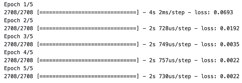

To perform regression tasks, the code provides a hybrid model that combines Long Short-Term Memory (LSTM) and Gated Recurrent Units (GRU) layers. The model is built using the Sequential class from the Keras library, allowing for a sequential layer-by-layer construction. A Sequential instance is created and assigned to the variable ‘regressorLG’. This instance will serve as the container for the model’s layers. Layers are then added to the ‘regressorLG’ model to define its architecture. A 50-unit LSTM layer is the first layer added. This layer is set to return sequences (return_sequences=True), and it expects input data with a shape of (X_train.shape[1], 1), where X_train.shap[1] represents the length of each input sequence. This layer is followed by a dropout layer. By dropping out a fraction of input units during training, this layer prevents overfitting. In this case, the dropout rate is set to 0.2. The model is then augmented with a GRU layer of 50 units. The GRU is a recurrent neural network (RNN) that captures temporal dependencies. The GRU layer uses the hyperbolic tangent (tanh) activation function. After the GRU layer, another dropout layer with the same dropout rate of 0.2 is added. This additional dropout layer contributes to regularizing the model and reducing overfitting. It produces a dense layer of one unit. This layer produces the final regression prediction.

The model is compiled using stochastic gradient descent (SGD). Several parameters are configured in the optimizer, including the learning rate (lr), decay, momentum, and Nesterov momentum. These parameters control how the optimizer adjusts the model’s weights during training. MSE is chosen as the loss function. The MSE is the difference between the predicted and actual values. It is commonly used for regression tasks. The model is then trained for five iterations on the training data (X_train and Y_train). Training is conducted in 150-person batches. During training, the model adjusts its weights to minimize the MSE loss between the predicted and actual values. A hybrid LSTM-GRU model is constructed using the provided code. By adding LSTM and GRU layers, applying dropout regularization, compiling the model with SGD optimizer and MSE loss, and training the model, the model’s architecture is defined.

dataset_total = pd.concat((dataset["High"][:'2017'],dataset["High"]['2018':]),axis=0)
inputs = dataset_total[len(dataset_total)-len(test_set) - 60:].values
inputs = inputs.reshape(-1,1)
inputs  = sc.transform(inputs)

As a result of this code, two different periods of the ‘dataset’ DataFrame are combined and prepared to be processed further.

The first line of code concatenates the “High” attribute values from two time periods: from the beginning of the DataFrame up to the year 2017 (‘dataset[“High”][:’2017']’) and from the year 2018 onwards (‘dataset[“High”][‘2018’:’]’). Using the ‘axis=0’ parameter, the ‘pd.concat’ function concatenates the data along the 0 axis (rows). The resulting concatenated data is stored in the ‘dataset_total’ variable. A portion of the ‘dataset_total’ variable is selected that corresponds to the length of the ‘test_set’ plus 60 additional values. In this case, the selection is made by using the slicing notation ‘[len(dataset_total)-len(test_set) — 60:]’. In the ‘len(dataset_total)-len(test_set) — 60’ expression, the starting index of the desired data is calculated. The ‘.values’ attribute converts the selected data into a NumPy array, which is then assigned to the ‘inputs’ variable. This is done by reshaping the array to have a shape of (-1, 1). The ‘-1’ indicates that the size of the dimension is inferred based on the length of the data and the other specified dimension, which is 1. Reshaping to (-1, 1) is often done to prepare the data for scaling or modeling purposes. In the fourth line, the MinMaxScaler object is used to scale the reshaped ‘inputs’ data. The ‘transform’ method of the scaler is called to perform the scaling operation, and the transformed data is reassigned to the ‘inputs’ variable.

To create ‘dataset_total’, this code concatenates the “High” attribute data from two different time periods into the ‘dataset’ DataFrame. It then selects a specific portion of the concatenated data, reshapes it, and applies scaling using the ‘sc’ MinMaxScaler object. Scaled data is stored in the ‘inputs’ variable for further analysis or modeling.

# Preparing X_test and predicting the prices
X_test = []
for i in range(60,119):
    X_test.append(inputs[i-60:i,0])
X_test = np.array(X_test)
X_test = np.reshape(X_test, (X_test.shape[0],X_test.shape[1],1))
LG_predicted_stock_price = regressorLG.predict(X_test)
LG_predicted_stock_price = sc.inverse_transform(LG_predicted_stock_price)

This code prepares the test data and makes predictions for the stock prices using a trained model. To store the test input sequences, the code creates an empty list, ‘X_test’. It then iterates over a range of indices from 60 to 118 (both inclusive) using a for loop. A slice of the input data is added to the ‘X_test’ list at each iteration. From index i-60 to index i, the slice represents 60 consecutive values. In the slice, only the values from the first column (index 0) of the input data are included. Each appended slice becomes an input sequence for testing. Using ‘np.array’, the ‘X_test’ list is converted into a NumPy array. This conversion is done to facilitate further processing and model input requirements. The next line reshapes the ‘X_test’ array to match the expected input shape.

A new shape is defined as (X_test.shape[0], X_test.shape[1], 1), where ‘X_test.shape[0]’ represents the number of test input sequences, ‘X_test.shape[1]’ represents the length of each sequence (60 in this case), and the additional dimension of 1 indicates each value in the sequence is treated individually. Based on the reshaped ‘X_test’ data, ‘regressorLG.predict’ function is used to make predictions. This function applies the trained ‘regressorLG’ model to the test data and returns the predicted values for the stock prices. The predicted stock prices are then inverse-transformed using the ‘sc’ MinMaxScaler object.

Obtaining the predicted prices in their original scale and units requires this step. The inverse-transformed predicted prices are stored in the ‘LG_predicted_stock_price’ variable for further analysis or evaluation. To summarize, this code creates input sequences from inputs. The model then reshapes the test data to match its input requirements, makes predictions on the reshaped data using the ‘regressorLG’ model, and obtains the predicted stock prices in their original scale using the ‘sc’ MinMaxScaler object. ‘LG_predicted_stock_price’ stores the predicted stock prices.

# Visualizing the results for GRU
plot_predictions(test_set,LG_predicted_stock_price)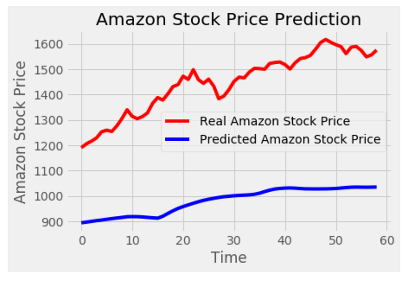

By plotting the actual and predicted stock prices, this code visualizes the results of the GRU model. The ‘plot_predictions’ function is called, passing ‘test_set’ (actual stock prices) and ‘LG_predicted_stock_price’ (predicted stock prices) as arguments. A line plot is generated inside the ‘plot_predictions’ function that displays actual stock prices in red and predicted stock prices in blue. The ‘test_set’ represents the x-axis values, which correspond to the time periods or data points, while ‘LG_predicted_stock_price’ represents the y-axis values, which indicate the stock prices predicted. Based on the results, the plot compares actual stock prices with the predicted stock prices. By visualizing the results, it becomes easier to assess the performance of the model in capturing the patterns and trends in the stock price data. To summarize, this code produces a plot comparing actual and predicted stock prices. Using the plot, you can evaluate the accuracy and effectiveness of the model’s predictions.