Hands-on Tutorial

Fixed Feature Extractor as the Transfer Learning Method for Image Classification Using MobileNet

Using transfer learning, you don’t need to build a convolutional neural network (CNN) from scratch

Nowadays, the growth of methods and algorithms in data science is increasing exponentially. Many companies begin adopting data science in their business. Many of them are for cost optimization, customer engagements, product development, etc. In several cases, the implementation leads to computer vision.

Further, computer vision has many implementations, such as image classification. As we all know, the development of its model from scratch requires high computer specifications and affects duration.

In this article, you will be introduced to the transfer learning concept and implementation using Python. Using transfer learning, you don’t need to make a CNN model from scratch for image classification but still has a good model performance. So, keep reading and try this tutorial by yourself!

Happy reading!

Background — it is my experience when I was at a university

Two years ago when I was at university, I faced an image classification problem in my national data mining competition. As a Statistics student, this field was too abstract for me — at that time, but I kept learning from the internet, and online courses and had a discussion with my friends (they were also my team) in the computer science department.

My team didn’t know about transfer learning, so we made a CNN model from scratch with only 10 epochs for 800 images that have 5 classes. or the information, we only had 3 hours for image preprocessing, model development, and pitch deck preparation. The result? My score was 4 out of 10 teams — only had 16.5% in mean average precision (mAP).

On the podium, I asked the first winner about the model they made. They told me about transfer learning and how it made them win the competition.

Using transfer learning, you don’t need to create a CNN from scratch

Transfer learning is an implementation of a model that has been trained with a large data set — known as a pre-trained model to another problem (but still related).

The concept is like between teacher and student. Teachers (in this case is a pre-trained model) try to transfer their knowledge to students (in this case is another problem). After the transfer process, students become smart and can solve the problem

The transfer learning in image classification appears along with the ImageNet competition in 2010. The competition uses 1281167 images for the training set, 50000 images for the validation set and 100000 images for the testing set. This image has 1000 classes.

Every year, the winner that successfully gets the highest model performance is announced. In 2021, the winner is CoAtNet-7 with an accuracy of 90.88%.

Transfer learning types

In transfer learning, there are three kinds of methods that can be used (depending on the problem statement). They are as follows.

Fixed feature extractor — the pre-trained model is used as a feature extractor in which the weights in the feature extraction layer are frozen while the fully connected layer is removed
Fine-tuning — it uses the architecture of a pre-trained model and initializes the weights in the feature extraction layer. It means the weights in the feature extraction layer are not frozen
Hybrid — the combination between fixed feature extractor and fine-tuning — some layers are frozen while the others are trained (their weights are initialized)

The question arises, how do we choose the method to be used in our problem? Which one is the right one? We should take a look at the following quadrant.

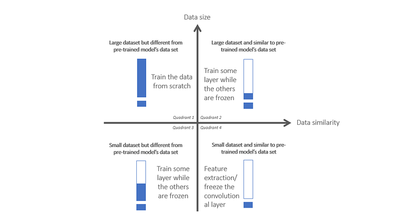
Transfer learning quadrant (Image by Author)

Quadrant 1 — large data size but has a small data similarity. In this case, better if we develop the model from scratch
Quadrant 2 — large data size but has a high data similarity. In this case, we should consider training some layers in the feature extraction layer while the others are frozen. The number of layers is debatable, it depends on the needs
Quadrant 3 — small data size but has a small data similarity. Similar to the quadrant 2 scenario
Quadrant 4 — small data size but has a high data similarity. In this case, we can implement the fixed feature extractor method for transfer learning

The more similar our data is to the pre-trained model’s data, the more layers are frozen

Why MobileNet?

Back to my story at university, the first winner told me that they used MobileNet as the pre-trained model. When the images in my competition are types of leaf, the MobileNet successfully got the best mAP, around ~85%. So, it’s good to start if we talk about MobileNet in this tutorial.

Moreover, based on M. Hollemans (2018), the MobileNet, in general, has some advantages. They are as follows

Light-weight model so it can reduce the computing resources
Commonly implemented in mobile device

These advantages must be paid with the weakness of model performance. The best accuracy for MobileNet V2 is around ~74.70%.

The real implementation of transfer learning

Firstly, we should download the data sets here. It has two classes (dogs and cats) with 8000 images for the training and 2000 images for the validation set. The Jupyter notebook file is in the last section of this article.

Set the folder and files as follows.

TRANSFER LEARNING
├── data
│    ├── train
│    │   ├── cats
│    │   │   ├── cat.1.jpg
│    │   │   ├── cat.2.jpg
│    │   │   ├── ...
│    │   │   └── cat.100.jpg
│    │   └── dogs
│    │       ├── dog.1.jpg
│    │       ├── dog.2.jpg
│    │       ├── ...
│    │       └── dog.100.jpg
│    └── validation
│        ├── cats
│        │   ├── cat.4001.jpg
│        │   ├── cat.4002.jpg
│        │   ├── ...
│        │   └── cat.4030.jpg
│        └── dogs
│            ├── dog.4001.jpg
│            ├── dog.4002.jpg
│            ├── ...
│            └── dog.4030.jpg
└── Transfer Learning - Feature Extraction.ipynb

If you haven’t installed Keras and Tensorflow on your computer yet, I recommend you to use Google Collabs in which the data set must be uploaded into Google Drive.

Note — the hands-on tutorial in this article is using Google Collabs

# Linear algebra calculation
import numpy as np
# To interact with operating system
import os
# Data visualization - matplotlib
import matplotlib.pyplot as plt
# Data visualization - plotnine
from plotnine import *
from plotnine import ggplot
import plotnine
# Tensorflow
import tensorflow as tf
from tensorflow.keras.preprocessing import image_dataset_from_directory
from tensorflow.keras.layers.experimental.preprocessing import RandomFlip, RandomRotation, Rescaling
from tensorflow.keras.applications import MobileNetV2
# Data manipulation
import pandas as pd
# Ignore warnings
import warnings
warnings.filterwarnings('ignore', category = FutureWarning)

In my Google Drive, the folder is TRANSFER LEARNING. From the root path, we connect it with training and validation folders.

# Mount the Google Drive to Google Collabs
from google.colab import drive
drive.mount('/content/gdrive')
# Set the root path
root_path = 'gdrive/MyDrive/TRANSFER LEARNING/'
# Directory path
train_dir = os.path.join(root_path, 'data/train')
validation_dir = os.path.join(root_path, 'data/validation')

To load the images from the directory, we use image_dataset_from_directory with following settings.

batch_size — number of images loaded in a single process (default: 32)
image_size — to resize images so they will have the same size

# Set batch size and image size
BATCH_SIZE = 32
IMG_SIZE = (160, 160)
# Load images for training set
train_dataset = image_dataset_from_directory(
                        train_dir,
                        shuffle = True,
                        batch_size = BATCH_SIZE,
                        image_size = IMG_SIZE
                )
# Load images for training set
validation_dataset = image_dataset_from_directory(
                        validation_dir,
                        shuffle = True,
                        batch_size = BATCH_SIZE,
                        image_size = IMG_SIZE
                      )

After the previous script has been run, try to visualize them using matplotlib. It ensures that the images are successfully loaded into Python env and the labels are true.

# Class names in training set
class_names = train_dataset.class_names
# Set the image size for visualization
plt.figure(figsize = (10, 10))
# Loop the images
for images, labels in train_dataset.take(1):
    for i in range(9):
        ax = plt.subplot(3, 3, i + 1)
        plt.imshow(images[i].numpy().astype('uint8'))
        plt.title(class_names[labels[i]])
        plt.axis('off')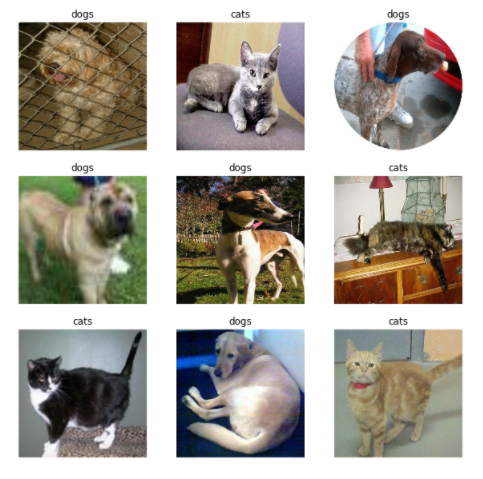

Sample images of training data (Image by Author)

Note — we consider use the scenario in the quadrant 4. Why? Because the images classes (dog and cat) are in ImageNet database (high data similarity) but with small data size

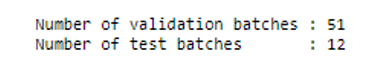
From the images in the validation set, we take out some to be the testing set. The size is determined as much as desired — depending on the needs.

# Create a testing set
val_batches = tf.data.experimental.cardinality(validation_dataset)
test_dataset = validation_dataset.take(val_batches // 5)
validation_dataset = validation_dataset.skip(val_batches // 5)
# Print out the validation and testing batch
print('Number of validation batches : {}'.format(
    tf.data.experimental.cardinality(validation_dataset))
)
print('Number of test batches       : {}'.format(
    tf.data.experimental.cardinality(test_dataset))
)

Batch for validation and testing set (Image by Author)

Based on the official Tensorflow documentation, the MobileNet requires the pixel size in [-1, 1] while ours is [0, 255]. So, we should rescale them using the following script (the script will be used in a pipeline).

# Rescale the image to [-1, 1]
rescale = Rescaling(scale = 1./127.5, offset = -1)

The MobileNet model is loaded and stored in base_model. We set include_top = False so that the fully connected layer will be excluded.

# Base model from the pre-trained model MobileNet V2
IMG_SHAPE = IMG_SIZE + (3, )
base_model = MobileNetV2(
                  input_shape = IMG_SHAPE,
                  include_top = False,
                  weights = 'imagenet'
              )

For the fixed feature extractor, the feature extraction layer is frozen. This is why we set the base_model.trainable = False.

# Freeze the feature extraction layer
base_model.trainable = False

In the model, we take the pipeline for data preprocessing — random flip, random scaling, and rescaling. Then, for the feature extraction layer, as previously mentioned, the pre-trained model of MobileNet is used.

The expected input layer is an image with dimensions (160, 160, 3). Then, because it’s the binary classification, we modify the fully connected layer for binary output.

# Set the input layer
inputs = tf.keras.Input(shape = (160, 160, 3))
# Data preprocessing
x = RandomFlip('horizontal')(inputs)
x = RandomRotation(0.2)(x)
x = Rescaling(scale = 1./127.5, offset = -1)(x)
# Feature extaction layer
x = base_model(x, training = False)
# Pooling layer
x = tf.keras.layers.GlobalAveragePooling2D()(x)
# Dropout layer
x = tf.keras.layers.Dropout(0.2)(x)
# Dense layer
outputs = tf.keras.layers.Dense(1)(x)
# Final model
model = tf.keras.Model(inputs, outputs)

The following image is the result of image preprocessing, such as random flip and random rotation. Its image preprocessing task is useful for generating random images so indirectly will prevent the overfitting problem in the model.

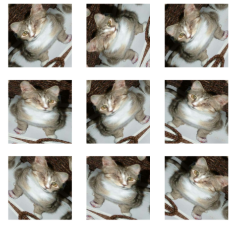
The result of image preprocessing — random flip and random rotation (Image by Author)

The model is finally compiled! We choose Adam as the optimizer and Binary Cross Entropy as the loss function. Then the metrics for evaluation are set to accuracy (balanced classes problem).

Note — you can determine the learning rate. For this tutorial, it is 0.0001

# Set the learning rate
base_learning_rate = 0.0001
# Compile the model
model.compile(
    optimizer = tf.keras.optimizers.Adam(
        learning_rate = base_learning_rate
    ),
    loss = tf.keras.losses.BinaryCrossentropy(
        from_logits = True
    ),
    metrics = ['accuracy']
)
# Model architecture
model.summary()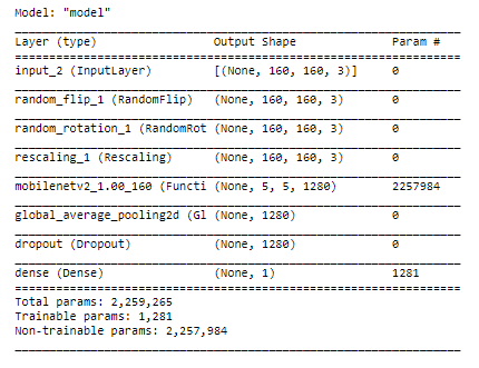

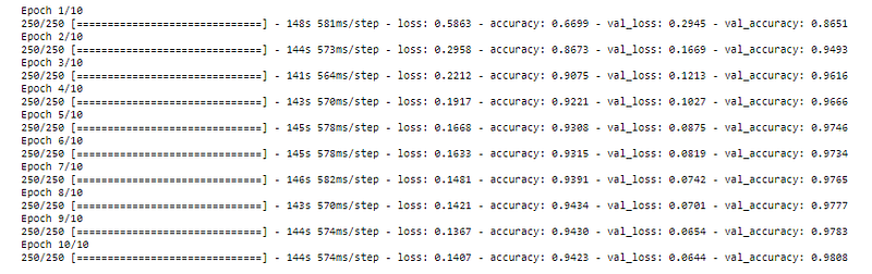
Final model architecture for image classification (Image by Author)

After compiling the model from the pre-trained model (feature extraction layer) and modification in the fully connected layer, we try to train the images in the training set using this model. The number of the epoch is set to 10 (it’s quite small but we will see the performance).

For the validation_data, we set to validation_dataset namely the images for model validation.

# Set the number of epochs
initial_epochs = 10
# Train the data
final_model = model.fit(
    train_dataset,
    epochs = initial_epochs,
    validation_data = validation_dataset
)

Training the final model using a pre-trained model of MobileNet (Image by Author)

The final_model contains the history of model performance in each epoch.

# Accuracy
accuracy_train = final_model.history['accuracy']
accuracy_val = final_model.history['val_accuracy']
# Loss
loss_train = final_model.history['loss']
loss_val = final_model.history['val_loss']

The information about model performance is parsed into a data frame. It will have 4 columns (Data, Epoch, Accuracy, Loss).

# Data type
data_type = ['Training'] * initial_epochs + ['Validation'] * initial_epochs
# Create a data frame
df = pd.DataFrame(
        data = {
            'Data': data_type,
            'Epoch': list(range(1, initial_epochs + 1)) * 2,
            'Accuracy': accuracy_train + accuracy_val,
            'Loss': loss_train + loss_val
        }
    )
# Set the categorical data
df['Epoch'] = df['Epoch'].astype('category')
# Show the data
df.head()

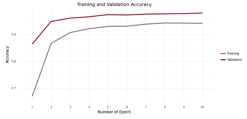
The history of model performance in each epoch (Image by Author)

The average accuracy in the training set is smaller than in the validation set. The training set has a 90.78% in average accuracy while the validation set has 96.47%. Moreover, it applies in each epoch in training.

# Data viz - accuracy
plotnine.options.figure_size = (10, 4.8)
(
    ggplot(data = df)+
    geom_line(aes(x = 'Epoch',
                  y = 'Accuracy',
                  color = 'Data',
                  group = 'Data'),
              size = 1.5,
              show_legend = True)+
    scale_color_manual(name = ' ', 
                       values = ['#80797c', '#981220'], 
                       labels = ['Training', 'Validation'])+
    labs(title = 'Training and Validation Accuracy')+
    xlab('Number of Epoch')+
    ylab('Accuracy')+
    theme_minimal()
)

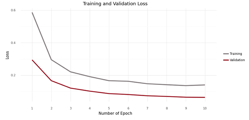
Training and validation accuracy of transfer learning (Image by Author)

Therefore, the average loss in the training set is greater than the validation set. The training set has 20.39% in the average loss while the validation set has 10.31%. It makes sense!

# Data viz - loss
plotnine.options.figure_size = (10, 4.8)
(
    ggplot(data = df)+
    geom_line(aes(x = 'Epoch',
                  y = 'Loss',
                  color = 'Data',
                  group = 'Data'),
              size = 1.5,
              show_legend = True)+
    scale_color_manual(name = ' ', 
                       values = ['#80797c', '#981220'], 
                       labels = ['Training', 'Validation'])+
    labs(title = 'Training and Validation Loss')+
    xlab('Loss')+
    ylab('Number of Epoch')+
    theme_minimal()
)

Training and validation loss of transfer learning (Image by Author)

After performing evaluation at the testing set, it produces an accuracy of 98.18%. Compared to training and validation, it can not be concluded that the model is overfitted. It means the model is quite robust in predicting the new images (for generalization). For 100 images, 98 will be predicted accurately.

# Get accuracy and loss for testing data
loss, accuracy = model.evaluate(test_dataset)
print('Test accuracy: {}'.format(accuracy))

The accuracy for a testing set (Image by Author)

The following script is used if we want to look at the sample prediction in the testing set. Even more, the result is visualized in images, so we can look at the model's robustness properly rather than only in numerical data (text).

# Retrieve a batch of images from the testing set
image_batch, label_batch = test_dataset.as_numpy_iterator().next()
predictions = model.predict_on_batch(image_batch).flatten()
# Apply a sigmoid since our model returns logits
predictions = tf.nn.sigmoid(predictions)
predictions = tf.where(predictions < 0.5, 0, 1)
# Visualize the prediction
plt.figure(figsize = (10, 10))
for i in range(9):
    # Get the labels
    text_pred = 'cats'
    if predictions[i] == 1:
        text_pred = 'dogs'
    
    # Return True/False for prediction
    stat = False
    if text_pred == class_names[predictions[i]]:
        stat = True
    
    # Show the images
    ax = plt.subplot(3, 3, i + 1)
    plt.imshow(image_batch[i].astype('uint8'))
    plt.title('Prediction: {} ({})'.format(text_pred, stat))
    plt.axis('off')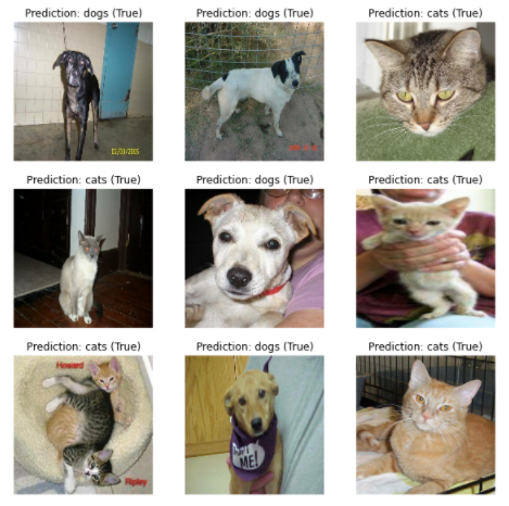

Predictions of the testing set (Image by Author)

References

[1] J. Brownlee. A Gentle Introduction to Transfer Learning for Deep Learning (2017). https://machinelearningmastery.com/.

[2] K. Dong, Y. Ruan, C. Zhou, Y. Li. 2020. MobileNetV2 Model for Image Classification. 2020 2nd International Conference on Information Technology and Computer Application (ITCA). Des 18 2020 — Des 20 2020. Guangzhou (CN). pp: 476–480.

[3] M. Hollemans. MobileNet Version 2 (2018). https://machinethink.net/.

[4] R. Adam. Transfer Learning: Solusi Deep Learning dengan Data Sedikit (2021). https://structilmy.com/.

[5] Tensorflow Developer. 2021. Transfer learning and fine-tuning [Internet]. [Downloaded on 2021 Oct 01]. Available at https://www.tensorflow.org/.

[6] W. Dai, Y. Dai, K. Hirota, Z. Jia. 2020. A Flower Classification Approach with MobileNetV2 and Transfer Learning. The 9th International Symposium on Computational Intelligence and Industrial Applications (ISCIIA2020). Oct 31 2020 — Nov 03 2020. Beijing (CN). pp: 1–5.

[7] Z. Dai, H. Liu, Q.V. Le, M. Tan. 2021. CoAtNet: Marrying Convolution and Attention for All Data Sizes [Internet]. [Downloaded on 2021 Oct 01]. Available at https://arxiv.org/.