
Fibonacci Mean-Reversion Strategy with the Slow Stochastic Oscillator
This article will present a simplistic application of several classical indicators to the financial markets, aiming to generate profits. As a preface, I am utilising Jupyter Notebook for writing and executing the commands on Tesla Closing Prices over a month long period.
A concise overview of this strategy is as follows: find medium and longer-term moving averages to assess if the market deviates significantly from its mean. If such deviation is observed, employ the slow stochastic oscillator to identify extremely overbought and oversold levels for entering positions. Subsequently, utilise fibonacci levels as take profit and stop loss targets. Note this is a basic application as standard setups for the indicators are assumed, better performance is probable if these are to be altered.
A main benefit of using these indicators over any machine learning technique is that they are not models skewed by training data that could result in overfitting and unrealistic performance.
The following packages were necessary to run the algorithm:
import yfinance as yf           # for the financial data
import numpy as np              # for the math
import pandas as pd             # for the data wrangling
import matplotlib.pyplot as plt # for the plots
Here is the first iteration of the algorithm with Stochastic Overbought and Oversold Entries at 80/20:
import yfinance as yf
import numpy as np
import pandas as pd
import matplotlib.pyplot as plt

def calculate_popular_moving_average(data, window):
    return data['Close'].rolling(window=window).mean()

def stochastic_oscillator(data, k_window=14, d_window=3):
    low_min = data['Low'].rolling(window=k_window).min()
    high_max = data['High'].rolling(window=k_window).max()

    k_percent = (data['Close'] - low_min) / (high_max - low_min) * 100
    d_percent = k_percent.rolling(window=d_window).mean()

    return k_percent, d_percent

def fibonacci_levels(high, low):
    diff = high - low
    return low, low + 0.236 * diff, low + 0.382 * diff, low + 0.618 * diff, high

def apply_strategy(data, account_size=1000, position_size=0.07):
    positions = []
    account_balance = account_size
    initial_balance = account_balance

    for i in range(2, len(data)):
        long_condition = (
            data['Close'][i] > data['Long_MA'][i]
            and data['Close'][i] > data['Medium_MA'][i]
            and data['Stochastic_K'][i] > 80
            and data['Stochastic_D'][i] > 80
        )

        short_condition = (
            data['Close'][i] < data['Long_MA'][i]
            and data['Close'][i] < data['Medium_MA'][i]
            and data['Stochastic_K'][i] < 20
            and data['Stochastic_D'][i] < 20
        )

        if long_condition or short_condition:
            high, low = data['High'][i], data['Low'][i]
            take_profit, _, _, _, stop_loss = fibonacci_levels(high, low)

            if long_condition:
                entry_type = 'Long'
                entry_price = data['Close'][i]
            elif short_condition:
                entry_type = 'Short'
                entry_price = data['Close'][i]

            position = {
                'Type': entry_type,
                'Entry Price': entry_price,
                'Take Profit': take_profit,
                'Stop Loss': stop_loss,
                'Entry Index': i,
                'Exit Index': None,
            }

            positions.append(position)

    # Set Exit Index for each position
    for i in range(1, len(positions)):
        positions[i - 1]['Exit Index'] = positions[i]['Entry Index']

    # Calculate returns
    returns = []
    for position in positions:
        if position['Exit Index']:
            if position['Type'] == 'Long':
                returns.append((data['Close'][position['Exit Index']] / position['Entry Price']) - 1)
            elif position['Type'] == 'Short':
                returns.append((position['Entry Price'] / data['Close'][position['Exit Index']]) - 1)

    # Plot cumulative performance
    cumulative_returns = np.cumprod(1 + np.array(returns))
    plt.figure(figsize=(10, 6))
    plt.plot(cumulative_returns, label='Cumulative Returns')
    plt.title('Cumulative Returns of the Strategy')
    plt.xlabel('Trade Number')
    plt.ylabel('Cumulative Returns')
    plt.legend()
    plt.show()

# Example usage
ticker = 'AAPL'
start_date = '2023-11-01'
end_date = '2023-12-01'

data = yf.download(ticker, start=start_date, end=end_date, interval='5m')

# Calculate moving averages
data['Long_MA'] = calculate_popular_moving_average(data, window=20)
data['Medium_MA'] = calculate_popular_moving_average(data, window=10)

# Calculate stochastic oscillator
data['Stochastic_K'], data['Stochastic_D'] = stochastic_oscillator(data)

# Apply strategy and plot cumulative returns
apply_strategy(data)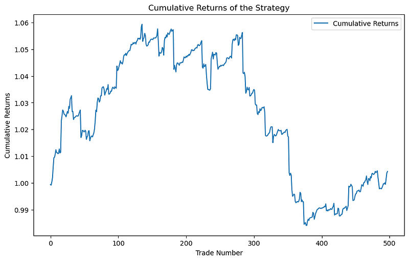
Over the month-long period, the strategy executed approximately 500 trades and yielded a marginal return. The initial profit run, followed by the subsequent loss run, could be a result of this algorithm overtrading. Consequently, I tightened the entry requirements by increasing the stochastic oscillator range to 90/10, as outlined below:
import yfinance as yf
import numpy as np
import pandas as pd
import matplotlib.pyplot as plt

def calculate_popular_moving_average(data, window):
    return data['Close'].rolling(window=window).mean()

def stochastic_oscillator(data, k_window=14, d_window=3):
    low_min = data['Low'].rolling(window=k_window).min()
    high_max = data['High'].rolling(window=k_window).max()

    k_percent = (data['Close'] - low_min) / (high_max - low_min) * 100
    d_percent = k_percent.rolling(window=d_window).mean()

    return k_percent, d_percent

def fibonacci_levels(high, low):
    diff = high - low
    return low, low + 0.236 * diff, low + 0.382 * diff, low + 0.618 * diff, high

def apply_strategy(data, account_size=1000, position_size=0.07):
    positions = []
    account_balance = account_size
    initial_balance = account_balance

    for i in range(2, len(data)):
        long_condition = (
            data['Close'][i] > data['Long_MA'][i]
            and data['Close'][i] > data['Medium_MA'][i]
            and data['Stochastic_K'][i] > 90
            and data['Stochastic_D'][i] > 90
        )

        short_condition = (
            data['Close'][i] < data['Long_MA'][i]
            and data['Close'][i] < data['Medium_MA'][i]
            and data['Stochastic_K'][i] < 10
            and data['Stochastic_D'][i] < 10
        )

        if long_condition or short_condition:
            high, low = data['High'][i], data['Low'][i]
            take_profit, _, _, _, stop_loss = fibonacci_levels(high, low)

            if long_condition:
                entry_type = 'Long'
                entry_price = data['Close'][i]
            elif short_condition:
                entry_type = 'Short'
                entry_price = data['Close'][i]

            position = {
                'Type': entry_type,
                'Entry Price': entry_price,
                'Take Profit': take_profit,
                'Stop Loss': stop_loss,
                'Entry Index': i,
                'Exit Index': None,
            }

            positions.append(position)

    # Set Exit Index for each position
    for i in range(1, len(positions)):
        positions[i - 1]['Exit Index'] = positions[i]['Entry Index']

    # Calculate returns
    returns = []
    for position in positions:
        if position['Exit Index']:
            if position['Type'] == 'Long':
                returns.append((data['Close'][position['Exit Index']] / position['Entry Price']) - 1)
            elif position['Type'] == 'Short':
                returns.append((position['Entry Price'] / data['Close'][position['Exit Index']]) - 1)

    # Plot cumulative performance
    cumulative_returns = np.cumprod(1 + np.array(returns))
    plt.figure(figsize=(10, 6))
    plt.plot(cumulative_returns, label='Cumulative Returns')
    plt.title('Cumulative Returns of the Strategy')
    plt.xlabel('Trade Number')
    plt.ylabel('Cumulative Returns')
    plt.show()

    # Plot Tesla data with entry and exit points
    plt.figure(figsize=(12, 8))
    plt.plot(data['Close'], label='Tesla Close Price', alpha=0.7)
    for position in positions:
        entry_index = position['Entry Index']
        exit_index = position['Exit Index']
        entry_price = position['Entry Price']
        exit_price = data['Close'][exit_index] if exit_index else None

        plt.scatter(data.index[entry_index], entry_price, marker='^', color='g', label='Entry Point')
        if exit_index:
            plt.scatter(data.index[exit_index], exit_price, marker='v', color='r', label='Exit Point')

    plt.title('Tesla Close Price with Entry and Exit Points')
    plt.xlabel('Date')
    plt.ylabel('Close Price')
    plt.show()

# Example usage
ticker = 'AAPL'
start_date = '2023-11-01'
end_date = '2023-12-01'

data = yf.download(ticker, start=start_date, end=end_date, interval='5m')

# Calculate moving averages
data['Long_MA'] = calculate_popular_moving_average(data, window=20)
data['Medium_MA'] = calculate_popular_moving_average(data, window=10)

# Calculate stochastic oscillator
data['Stochastic_K'], data['Stochastic_D'] = stochastic_oscillator(data)

# Apply and plot the strategy
apply_strategy(data)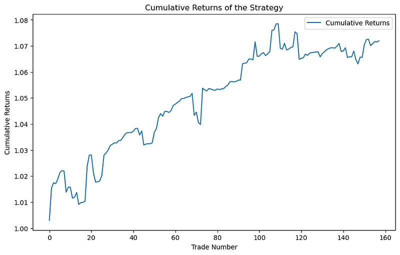
This iteration has a definite improvement on the first, resulting from tighter entry requirements when the stock is overbought/oversold. Clearly adjusting the entry criteria with the slow stochastic oscillator is a determining factor in the performance of this strategy .
The +7% return is encouraging for such a simple application. Note that trade fees; slippage and spreads, are disregarded for simplicity and are likely to have a significant effect on an algorithmic strategy that employs as many trades as this. Improvements that could be made to this strategy include; optimising the fibonacci take profit / stop loss levels, increasing the size of the data set, optimising position sizing for stronger set ups, having better defined trend indicators.
An overview of each component in this strategy is provided below:
Moving Averages: The strategy calculates two moving averages: a long-term moving average (Long_MA) with a window of 20 periods and a medium-term moving average (Medium_MA) with a window of 10 periods. It uses these moving averages to determine the trend direction.
Stochastic Oscillator: The strategy calculates the slow stochastic oscillator with a %K window of 14 and a %D window of 3. The stochastic oscillator measures the momentum and overbought/oversold conditions of the asset’s price. Values above 90 indicate overbought conditions, and values below 10 indicate oversold conditions.
Fibonacci Levels: The strategy uses Fibonacci retracement levels to set take-profit and stop-loss levels for trades. These levels are calculated based on the high and low prices.
Trade Conditions: Long Trades: The strategy initiates a long trade when the following conditions are met: The closing price is above both the long-term and medium-term moving averages. The slow stochastic %K and %D are both above 90, indicating overbought conditions. Short Trades: The strategy initiates a short trade when the following conditions are met: The closing price is below both the long-term and medium-term moving averages. The slow stochastic %K and %D are both below 10, indicating oversold conditions.
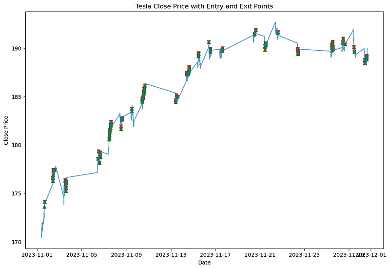
Entry and Exit Points: For each trade, the strategy records the entry point when the conditions are met. The strategy waits until the price hits the take-profit or stop-loss level to record the exit point. Exit points are used to calculate returns.
Position Sizing: The strategy assumes a fixed position size of 7% of the account for each trade.


