CLIP: The Most Influential AI Model From OpenAI — And How To Use It

Find out how the model works — coding example included

What do the recent AI breakthroughs, DALLE[1] and Stable Diffusion[2] have in common?

They both use components of CLIP’s[3] architecture. Hence, if you want to grasp how those models work, understanding CLIP is a prerequisite.

Besides, CLIP has been used to index photos on Unsplash.

But what does CLIP do, and why it’s a milestone for the AI community?

Let’s dive in!

CLIP — An Overview

CLIP stands for Constastive Language-Image Pretraining:

CLIP is an open source, multi-modal, zero-shot model. Given an image and text descriptions, the model can predict the most relevant text description for that image, without optimizing for a particular task.

Let’s break down this description:

• Open Source: The model is created and open-sourced by OpenAI. We will later see a programming tutorial on how to use it.
• Multi-Modal: Multi-Modal architectures leverage more than one domain to learn a specific task. CLIP combines Natural Language Processing and Computer Vision.
• Zero-shot: Zero-shot learning is a way to generalize on unseen labels, without having specifically trained to classify them. For example, all ImageNet models are trained to recognize 1000 specific classes. CLIP is not bound by this limitation.
• Constastive Language: With this technique, CLIP is trained to understand that similar representations should be close to the latent space, while dissimilar ones should be far apart. This will become more clear later with an example.

Fun facts about CLIP:

• CLIP is trained using a staggering amount of 400 million image-text pairs. For comparison, the ImageNet dataset contains 1.2 million images.
• The final tuned CLIP model was trained on 256 V100 GPUs for two weeks. For an on-demand training on AWS Sagemaker, this would cost at least 200k dollars!
• The model uses a minibatch of 32,768 images for training.

CLIP in Action

Let’s demonstrate visually what CLIP does. We will later show a coding example in more detail.

First, we select a free image from Unsplash:

Next, we provide CLIP with the following prompts:

• ‘a girl wearing a beanie’.
• ‘a girl wearing a hat’.
• ‘a boy wearing a beanie’.
• ‘a girl riding a bike’.
• ‘a dog’.

Obviously, the first description better describes the image.

CLIP automatically finds which text prompt describes the image optimally by assigning a normalized probability. We get:

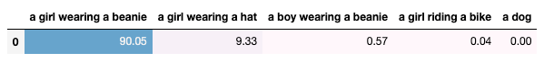
The model successfully locates the most fitting image description.

Also, CLIP can accurately recognize classes and objects that it has never seen before.

If you have a large image dataset and you want to label those images into specific classes/categories/descriptions, CLIP will do this automatically for you!

Next, we will show how CLIP works.

CLIP Architecture

CLIP is a deep learning model that uses novel ideas from other successful architectures and introduces some of its own.

Let’s start with the first part, the Contrastive Pre-training:

Contrastive Pre-training

Figure 1 shows an overview of the Contrastive Pre-training process.

Assume we have a batch of N images paired with their respective descriptions e.g. <image1, text1>, <image2, text2>, <imageN, textN>.

Contrastive Pre-training aims to jointly train an Image and a Text Encoder that produce image embeddings [I1, I2 … IN] and text embeddings [T1, T2 … TN], in a way that:

• The cosine similarities of the correct <image-text> embedding pairs <I1,T1>, <I2,T2> (where i=j) are maximized.
• In a contrastive fashion, the cosine similarities of dissimilar pairs <I1,T2>, <I1,T3>… <Ii,Tj> (where i≠j) are minimized.

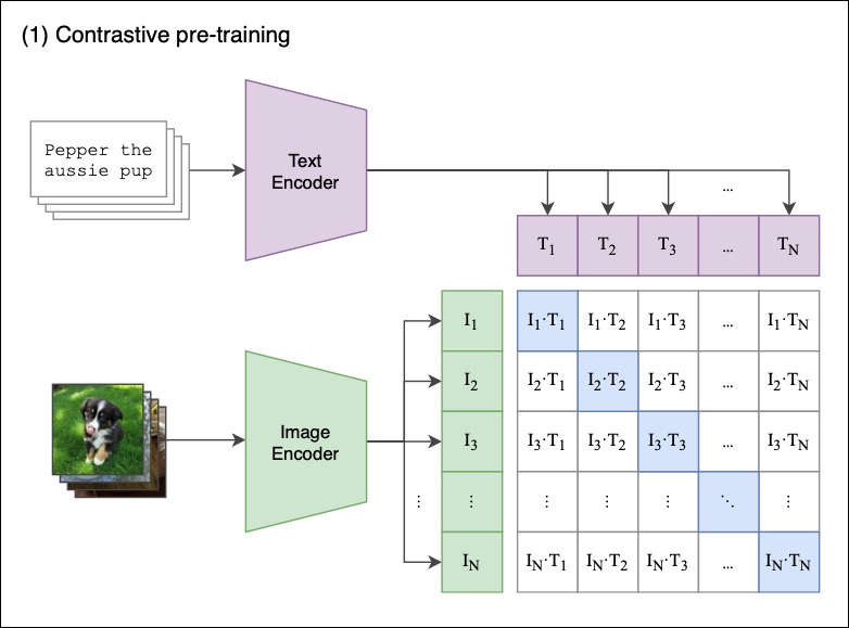
Let’s see what happens step-by-step:

1. The model receives a batch of N pairs.
2. The Text Encoder is a standard Transformer model with GPT2-style modifications[4]. The Image Encoder can be either a ResNet or a Vision Transformer[5].
3. For every image in the batch, the Image Encoder computes an image vector. The first image corresponds to the I1 vector, the second to I2 , and so on. Each vector is of size de, where de is the size of the latent dimension. Hence, the output of this step is N X de matrix.
4. Similarly, the textual descriptions are squashed into text embeddings [T1, T2 … TN], producing a N X de matrix.
5. Finally, we multiply those matrices and calculate the pairwise cosine similarities between every image and text description. This produces an N X N matrix, shown in Figure 1.
6. The goal is to maximize the cosine similarity along the diagonal — these are the correct <image-text> pairs. In a contrastive fashion, off-diagonal elements should have their similarities minimized (e.g I1 image is described by T1 and not by T2 , T2 ,T3 etc).

A few extra remarks:

• The model uses the symmetric cross-entropy loss as its optimization objective. This type of loss minimizes both the image-to-text direction as well as the text-to-image direction (remember, our contrastive loss matrix keeps both the <I1,T2> and <I2,T1> cosine similarities).
• Contrastive Pre-training is not entirely new. It was introduced in previous models and was adapted by CLIP[6].

Zero-Shot Classification

We have now pre-trained our Image and Text Encoders, and we are ready for Zero-Shot Classification.

The baseline First, let’s provide some context. How few-shot classification was implemented in the Pre-Transformer era?

It’s simple[7]:

• Download a high-performance pretrained CNN such as ResNet, and use it for feature extraction to get the image features.
• Then, use these features as an input to a standard classifier (such as Logistic Regression). The classifier is trained in a supervised way, where the image labels serve as the target variable (Figure 2).
• If you opt for K-shot learning, your training set during the classification phase should contain only K instances of each class.
• When K<10 , the task is referred to as few-shot classification learning. Accordingly, for K=1 we have one-shot classification learning. If we use all the available data, this is a fully-supervised model (the old-fashioned way).

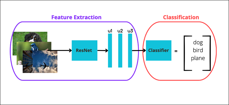
Notice the keyword ‘supervised’ above — the classifier should know the class labels beforehand. Using an image extractor paired with a classifier is also known as linear probe evaluation.

CLIP’s competitive advantage The process of how CLIP performs zero-shot classification is shown in Figure 3:

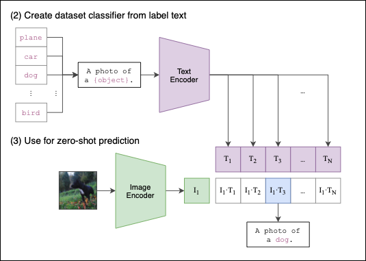
Again, the process is straightforward:

First, we provide a set of text descriptions such as a photo of a dog or a cat eating an ice-cream (whatever we think best describes one or more images). These text descriptions are encoded into text embeddings.

Then, we do the same with an image — the image is encoded into an image embedding.

Finally, CLIP computes the pairwise cosine similarities between the image and the text embeddings. The text prompt with the highest similarity is chosen as the prediction.

Of course, we can input more than one image. CLIP cleverly caches the input text embeddings, so they don’t have to be recomputed for the rest of the input images.

And that’s it! We have now concluded how CLIP works end-to-end.

The Problem Of Finding Data

CLIP uses 30 public datasets for pre-training. Fitting a large language model with a tremendous amount of data is important.

However, it is difficult to find robust datasets with paired image-textual descriptions. Most public datasets, such as CIFAR, are images with just one-single-word labels — these labels are the target class. But CLIP was created to use full textual descriptions.

To overcome this discrepancy, the authors did not exclude those datasets. Instead, they performed some feature engineering: Single word labels, such as a bird, or acar were converted to sentences: a photo of a dog or a photo of bird. On the Oxford-IIIT Pets dataset, the authors used the prompt: A photo of a {label}, a type of pet.

For additional info on pretraining techniques, check the original paper[3].

The Impact Of CLIP In AI

Initially, we claimed that CLIP is a milestone for the AI community.

Let’s see why:

1. Superior performance as a Zero-Shot classifier

CLIP is a zero-shot classifier, so it makes sense to first test CLIP against few-shot learning models.

Thus, the authors tested CLIP against models that consist of a linear classifier on top of a high-quality pre-trained model, such as a ResNet.

The results are shown in Figure 4:

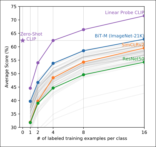
CLIP significantly outperforms the other classifiers.

Also, CLIP was able to match the performance of the 16-shot linear classifier BiT-M. To put it differently, the BiT-M’s classifier had to train on a dataset of at least 16 examples per class to match CLIP’s score — and CLIP achieves the same score without requiring fine-tuning.

Interestingly, the authors evaluated CLIP as a linear probe: They used only the CLIP’s Image Encoder to get the image features and fed them into a linear classifier — just like the other models. Even with this setup, CLIP’s few-shot-learning capabilities are outstanding.

2. Unparallel robustness to Distribution Shift

Distribution shift is a big deal, especially for machine learning systems in production.

Note: You may know distribution shift as concept drift, although technically they are not the same.

Distribution Shift is a phenomenon that occurs when the data a model was trained with changes over time. Thus, as time passes, the model’s efficiency degrades and predictions become less accurate.

In fact, distribution shift is not something unexpected — it will happen. Question is, how to detect this phenomenon early, and what actions are required to ‘recalibrate’ your model? This is not easy to solve and depends on many factors.

Fortunately, new research on AI heads towards creating models resilient to distribution shift.

That’s why the authors put CLIP’s robustness to the test. The results are displayed in Figure 5:

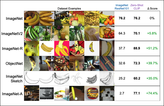
Two things here about CLIP have substantial importance:

1. CLIP achieves the same accuracy as a SOTA ResNet model on ImageNet, even though CLIP is a zero-shot model.
2. Apart from the original ImageNet, we have similar datasets that serve as a distribution shift benchmark. It seems that ResNet is struggling with those datasets. However, CLIP can handle unknown images very well — in fact, the model maintains the same level of accuracy theroughout all the variations of ImageNet!

3. Computational efficiency

Before GPT-2, computational efficiency was taken for granted (sort of).

Nowadays, in the era where a model takes weeks to train with hundreds of 8k dollar GPUs, the computational efficiency issue is addressed more seriously.

CLIP is a more computational-friendly architecture. Part of this success is because CLIP uses a Vision Transformer as the default Image Encoder component. The results are shown in Figure 6:

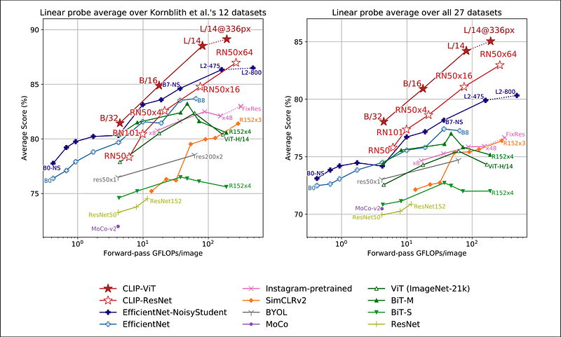
Clearly, CLIP is better able to utilize hardware resources compared to other models. This also translates to saving extra money when training on cloud services such as AWS Sagemaker. Additionally, Figure 6 shows that CLIP offers better scalability in terms of hardware operations vs accuracy score compared to other models.

There is still the issue of data efficiency. The authors show that CLIP is more data-efficient than similar models in a zero-shot setting. But, they do not address CLIP’s data efficiency in the pretraining phase. However, there is probably not much to do in this area, since CLIP uses two types of Transformers — and Transformers are data-hungry models by their nature.

4. Increased research interest

CLIP’s success sparked an interest in text-to-image models and popularized the Contrastive Pre-training method.

Apart from DALLE and Stable Diffusion, we can use CLIP as a Discriminator in GANs.

Moreover, the release of CLIP inspired similar CLIP-based publications that expand on the model’s features, such as DenseCLIP[8] and CoCoOp[9].

Also, Microsoft released X-CLIP[10], a minimal extension of CLIP for video-language understanding.

Bonus Info: A Pictionary-like app, called paint.wtf, uses CLIP to rank your drawings. Give it a try — it’s super fun!

How To Use CLIP — Coding Example

Next, we will show how to use CLIP using the HugginFaces Library.

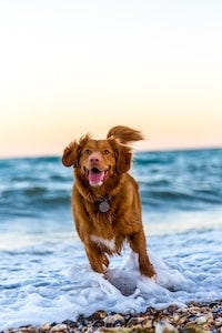
First, let’s select 3 images from Unsplash. We used the first earlier:

We will use the following libraries:

Next, we load the CLIP model’s weights, tokenizer image processor:

Also, we load the above Unsplash images in Python:

Finally, we provide CLIP with some text prompts.

The goal is to let CLIP classify the 3 Unsplash images into specific text descriptions. Notice that one of them is misleading — let’s find out if we can confuse the model:

The model successfully classifies all 3 images!

Notice two things:

1. CLIP can understand multiple entities along with their actions in each image.
2. CLIP assigns to each image the most specific description. For instance, we can describe the second image both as ‘a dog’ and ‘a dog at the beach’. However, the model correctly decides the ‘a dog’ phrase better describes the second image because there is no beach.

Feel free to play around with this example. The full example is here. Use your images with text descriptions and discover how CLIP works.

Limitations and Future Work

While CLIP is a revolutionary model, there is still room for improvement. The authors point out the areas where there is potential for further progress.

• Accuracy score: CLIP is a state-of-the-art zero-shot classifier that directly challenges task-specific trained models. The fact that CLIP matches the accuracy of a fully-supervised ResNet101 on ImageNet is phenomenal. However, there are still supervised models that achieve even higher scores. The authors stress that CLIP can probably achieve higher scores given its amazing scalability, but that would require an astronomical amount of computer resources.
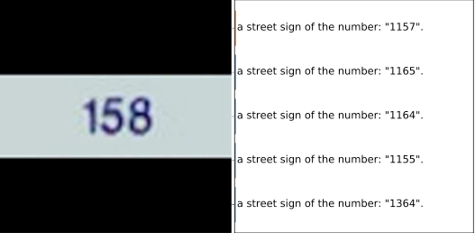
• Polysemy: The authors state that CLIP suffers from polysemy. Sometimes, the model cannot differentiate the meaning of some words due to a lack of context. Remember, we mentioned earlier that some images are tagged with just a class label and not a full-text prompt. The authors provide an example: In the Oxford-IIIT Pet dataset, the word ‘boxer’ refers to a dog breed, but other images perceive ‘boxer’ as an athlete. Here, the culprit is the quality of data and not the model itself.
• Task-specific learning: While CLIP can distinguish complex image patterns, the model fails with some trivial tasks. For example, the model struggles with handwritten digit recognition tasks (Figure 7). The authors attribute this type of misclassification to a lack of handwritten digits in the training datasets.

Closing Remarks

CLIP is without a doubt, a significant model for the AI community.

Essentially, CLIP paved the way for the new generation of text-to-image models that revolutionized AI research. And of course, don’t forget that this model is open-source.

Last but not least, there is lots of room for improvement. Throughout the paper, the authors imply that many of CLIP’s limitations are due to lower-quality training data.

Thank you for reading!

I write an in-depth analysis of an impactful paper on AI once a month. Stay connected!

• Subscribe to my newsletter!
• Follow me on Linkedin!
• Join Medium! (Affiliate Link)

References

1. Aditya Ramesh et al. Hierarchical Text-Conditional Image Generation with CLIP Latents (April 2022)
2. Robin Rombach et al. High-Resolution Image Synthesis with Latent Diffusion Models (April 2022)
3. Alec Radford et al. Learning Transferable Visual Models From Natural Language Supervision (Feb 2021)
4. Alec Radford et al. Language Models are Unsupervised Multitask Learners (2019)
5. Dosovitskiy et al. An Image is Worth 16x16 Words: Transformers for Image Recognition at Scale (2020)
6. Yuhao Zhang et al. CONTRASTIVE LEARNING OF MEDICAL VISUAL REPRESENTATIONS FROM PAIRED IMAGES AND TEXT (2020)
7. Tian, Y et al. Rethinking few-shot image classification: a good embedding is all you need? (2020)
8. Yongming Rao et al. DenseCLIP: Language-Guided Dense Prediction with Context-Aware Prompting
9. Kaiyang Zhou et al. Conditional Prompt Learning for Vision-Language Models (Mar 2022)
10. Bolin Ni et al. Expanding Language-Image Pretrained Models for General Video Recognition (August 2022)