TensorFlow Model Training Using GradientTape

Use of GradientTape to Update the Weights

TensorFlow is arguably the most popular library for deep learning. I wrote so many tutorials on TensorFlow before and still continuing. TensorFlow is very well organized and easy to use package where you do not need to worry about model development and model training too much. Pretty much most of the stuff is taken care of by the package itself. That is probably the reason why it has gotten so popular in the industry. But at the same time, sometimes it is nice to have control over the behind-the-scenes functionalities. It gives you a lot of power to experiment with the models. If you are job seeker, some extra knowledge may give you an edge.

Previously, I wrote an article on how to develop custom activation functions, layers, and loss functions. In this article, we will see how you can train the model manually and update the weights yourself. But don’t worry. You don’t have to remember the differential calculus all over again. We have GradientTape() method available in TensorFlow itself to take care of that part.

If GradientTape() is totally new to you, please feel free to check this exercises on GradientTape() that shows you, how GradientTape() works: Introduction to GradientTape in TensorFlow — Regenerative (regenerativetoday.com)

Data Preparation

In this article we work on a simple classification algorithm in TensorFlow using GradientTape(). Please download the dataset from this link:

Heart Failure Prediction Dataset (kaggle.com)

This dataset has an open database license.

These are the necessary imports:

import tensorflow as tf
from tensorflow.keras.models import Model
from tensorflow.keras.layers import Dense, Input
import numpy as np
import matplotlib.pyplot as plt
import matplotlib.ticker as mticker
import pandas as pd
from sklearn.model_selection import train_test_split
from sklearn.metrics import confusion_matrix
import itertools
from tqdm import tqdm
import tensorflow_datasets as tfds

Creating the DataFrame with the dataset:

import pandas as pd
df = pd.read_csv('heart.csv')
df

Output:

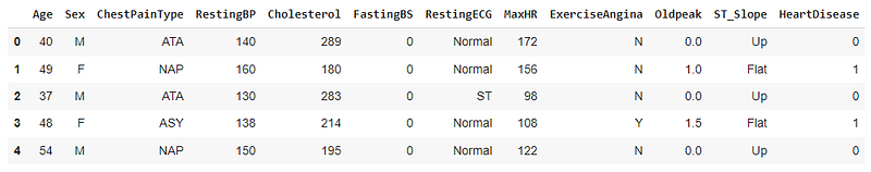
As shown in the picture above, there are multiple columns with string data type. Let’s check the data types of all the columns in the dataset:

df.dtypes

Output:

Age                 int64
Sex                object
ChestPainType      object
RestingBP           int64
Cholesterol         int64
FastingBS           int64
RestingECG         object
MaxHR               int64
ExerciseAngina     object
Oldpeak           float64
ST_Slope           object
HeartDisease        int64
dtype: object

As you are here, I can assume that you know the machine learning basics and already have learned that the data types need to be numeric for TensorFlow.

This code below loops through the columns and if the data type of a column is ‘object’, it changes that to numeric data.

for col in df.columns:
  if df[col].dtype == 'object':
    df[col] = df[col].astype('category').cat.codes

All the columns have become the numeric type now. Define the training features and target variable to move forward with the model:

X = df.drop(columns = 'HeartDisease')
y = df['HeartDisease']

We should keep a part of the dataset to evaluate the model. So we will use the train_test_split method here:

train, test = train_test_split(df, test_size=0.4)

Before diving into the model development part, it is also necessary to scale the data. I am using standard scaling method here that requires mean and standard deviation. Remember, we need the mean and standard deviation of the training data only. To scale the test data, the mean and standard deviation of training data needs to be used again as we shouldn’t reveal any information about the test data to the model.

We will use the .describe() method to find out the statistical parameters of each column of the training data:

train_stats = train.describe()
train_stats.pop('HeartDisease')
train_stats = train_stats.transpose()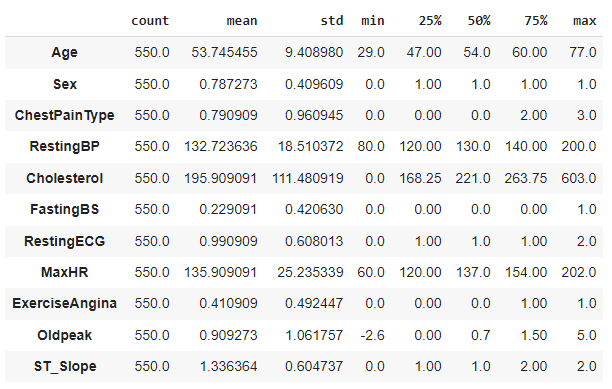

We have the parameters for scaling now.

Target variables for training and testing data need to be separated here:

y_train = train.pop('HeartDisease')
y_test = test.pop('HeartDisease')

The following function is defined to scale one column of a dataset using the standard scaling formula:

def norm(x):
  return (x - train_stats['mean']) / train_stats['std']

Using the function ‘norm’ scaling both training and testing data:

X_train_norm = norm(train)
X_test_norm = norm(test)

If you check the X_train_norm and X_test_norm, they are actually arrays. Converting them to tensors here:

train_dataset = tf.data.Dataset.from_tensor_slices((X_train_norm.values, y_train.values))
test_dataset = tf.data.Dataset.from_tensor_slices((X_test_norm.values, y_test.values))

Shuffling the datasets by each batch where batch_size is set to be 32:

batch_size = 32
train_dataset = train_dataset.shuffle(buffer_size = len(train)).batch(batch_size).prefetch(1)
test_dataset = test_dataset.batch(batch_size=batch_size).prefetch(1)

Model Development

We will take a simple TensorFlow model for this as the dataset is so simple. The model is defined as a function base_model where two fully connected Dense layers of 64 neurons and one output layers are added. In the last line, the function base_model called and saved in a variable called ’model’.

def base_model():
  inputs = tf.keras.layers.Input(shape = len(train.columns))
  x = tf.keras.layers.Dense(64, activation='LeakyReLU')(inputs)
  x = tf.keras.layers.Dense(64, activation='LeakyReLU')(x)
  outputs = tf.keras.layers.Dense(1, activation='sigmoid')(x)

  model = tf.keras.Model(inputs=inputs, outputs = outputs)
  return model

model = base_model()

I chose RMSprop optimizer and BinaryCrossentropy() loss function for this example. Please feel free to use any other Optimizer of your choice.

optimizer = tf.keras.optimizers.legacy.RMSprop(learning_rate=0.001)
loss_object = tf.keras.losses.BinaryCrossentropy()

Model Training

The GradientTape part is going to be useful in the model training part. During the model training we need the differentiation to update the weights. The function below will use the GradientTape to calculate the gradients. First it calculates the outputs using the model which is called the logits. Using the true label and predicted label, loss was calculated.

Then the gradients were calculated taking the differential of loss with respect to the weights and applied the gradients to the optimizers:

def gradient_calc(optimizer, loss_object, model, X, y):
  with tf.GradientTape() as tape:
    logits = model(X)
    loss = loss_object(y_true=y, y_pred=logits)

  gradients = tape.gradient(loss, model.trainable_weights)
  optimizer.apply_gradients(zip(gradients, model.trainable_weights))

  return logits, loss

The next function is to train the network for one epoch. Training one epoch includes:

the process of gradient calculation and applying as in the ‘gradient_calc’ function,

saving the losses and

updating the true label to the predicted label by the model after one epoch.

def training_one_epoch(train_data, optimizer, loss_object, model):
  losses = []
  for step, (x_batch, y_batch) in enumerate(train_data):
    logits, loss = gradient_calc(optimizer, loss_object, model, x_batch, y_batch)
    losses.append(loss)

    logits = tf.round(logits)
    logits = tf.cast(logits, 'int64')

    train_acc_metric.update_state(y_batch, logits)
  return losses

One more function is necessary before we start the model training. That is the function for the validation loss. This function is pretty self explanatory. It calculates the validation loss using the true label and the predicted label, append the loss to the list of losses, finally updates the true label for the validation data to the new calculated labels.

def validation_loss():
  losses = []
  for val_x, val_y in test_dataset:
    val_logits = model(val_x)
    val_loss = loss_object(y_true = val_y, y_pred=val_logits)
    losses.append(val_loss)

    val_logits = tf.cast(tf.round(model(val_x)), 'int64')

    val_acc_metric.update_state(val_y, val_logits)
  return losses

For this model I decided to use the accuracy as the evaluation metric. Calling the BinaryAccuracy() method for both training and validation:

train_acc_metric = tf.keras.metrics.BinaryAccuracy()
val_acc_metric = tf.keras.metrics.BinaryAccuracy()

It’s model training time. I am training this model for 60 epochs. We will loop through the epochs,

we can get the training losses by calling the ‘training_one_epoch’ function in each epoch, and validation loss by calling the ‘validation_loss’ function. These functions will provide up with a list of losses for each epoch because they will calculate the losses for all the data separately. We will take the mean of all the losses to get only one loss per epoch for both training and validation.

epochs = 60
val_losses, train_losses = [], []

for epoch in range(epochs):
  print('Start of epoch %d' % (epoch,))

  train_loss = training_one_epoch(train_dataset, optimizer, loss_object, model)

  train_acc = train_acc_metric.result()
  val_loss = validation_loss()

  val_acc = val_acc_metric.result()

  train_losses_mean = np.mean(train_loss)
  val_losses_mean = np.mean(val_loss)

  val_losses.append(val_losses_mean)
  train_losses.append(train_losses_mean)

  print('\n Epcoh %s: Training loss: %.3f  Validation Loss: %.3f, Training Accuracy: %.3f, Validation Accuracy %.3f' % (epoch, float(train_losses_mean), float(val_losses_mean), float(train_acc), float(val_acc)))

  train_acc_metric.reset_states()
  val_acc_metric.reset_states()

Here is the output for last few epochs:

Epcoh 56: Training loss: 0.204  Validation Loss: 0.333, Training Accuracy: 0.922, Validation Accuracy 0.872
Start of epoch 57

 Epcoh 57: Training loss: 0.219  Validation Loss: 0.350, Training Accuracy: 0.913, Validation Accuracy 0.878
Start of epoch 58

 Epcoh 58: Training loss: 0.203  Validation Loss: 0.335, Training Accuracy: 0.929, Validation Accuracy 0.872
Start of epoch 59

 Epcoh 59: Training loss: 0.205  Validation Loss: 0.349, Training Accuracy: 0.933, Validation Accuracy 0.875

After the 60 epochs, we got 93.3% accuracy for training data and 87.5% aacuracy for the validation data. Please feel free to train the model for more epochs to check if you can improve the accuracy scores. But please be aware of the overfitting issue.

Conclusion

In this article, we worked on an example to learn how to manually train the model instead of using the model.compile() method. This should give you better understanding of the TensorFlow library itself and how exactly model training works in TensorFlow.

More Reading

How to Define Custom Layer, Activation Function, and Loss Function in TensorFlow | by Rashida Nasrin Sucky | Towards Data Science (medium.com)

Anomaly Detection in TensorFlow and Keras Using the Autoencoder Method | by Rashida Nasrin Sucky | Sep, 2023 | Towards Data Science (medium.com)

Using a Keras Tuner for Hyperparameter Tuning of a TensorFlow Model | by Rashida Nasrin Sucky | Towards AI (medium.com)

Implementation of a Siamese Network in Keras and TensorFlow | by Rashida Nasrin Sucky | Towards Data Science (medium.com)

Complete Implementation of a Mini VGG Network for Image Recognition | by Rashida Nasrin Sucky | Towards Data Science (medium.com)