Extract Features, Visualize Filters and Feature Maps in VGG16 and VGG19 CNN Models

Learn How to Extract Features, Visualize Filters and Feature Maps in VGG16 and VGG19 CNN Models

Keras provides a set of deep learning models that are made available alongside pre-trained weights on ImageNet dataset. These models can be used for prediction, feature extraction, and fine-tuning. Here I’m going to discuss how to extract features, visualize filters and feature maps for the pretrained models VGG16 and VGG19 for a given image.

Extract Features with VGG16

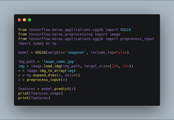
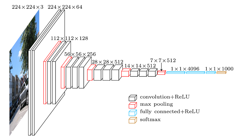
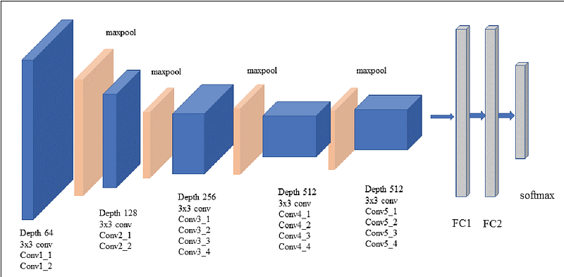
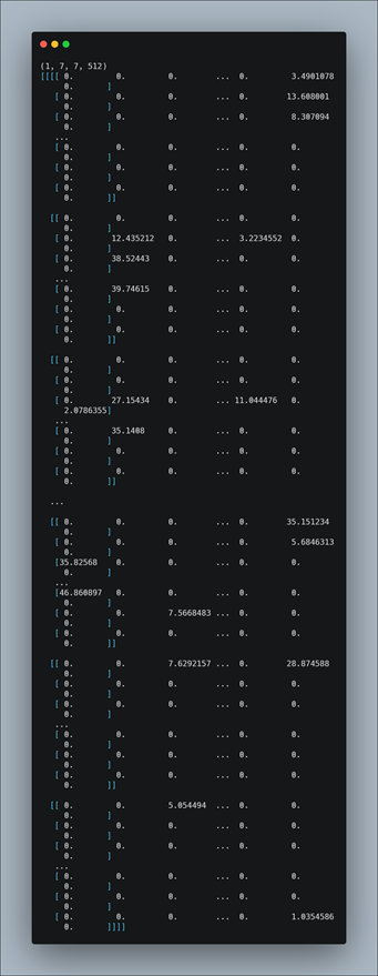
Here we first import the VGG16 model from tensorflow keras. The image module is imported to preprocess the image object and the preprocess_input module is imported to scale pixel values appropriately for the VGG16 model. The numpy module is imported for array-processing. Then the VGG16 model is loaded with the pretrained weights for the imagenet dataset. VGG16 model is a series of convolutional layers followed by one or a few dense (or fully connected) layers. Include_top lets you select if you want the final dense layers or not. False indicates that the final dense layers are excluded when loading the model. From the input layer to the last max pooling layer (labeled by 7 x 7 x 512) is regarded as feature extraction part of the model, while the rest of the network is regarded as classification part of the model. After defining the model, we need to load the input image with the size expected by the model, in this case, 224×224. Next, the image PIL object needs to be converted to a NumPy array of pixel data and expanded from a 3D array to a 4D array with the dimensions of [samples, rows, cols, channels], where we only have one sample. The pixel values then need to be scaled appropriately for the VGG model. We are now ready to get the features.

Extract Features from an Arbitrary Intermediate Layer with VGG16

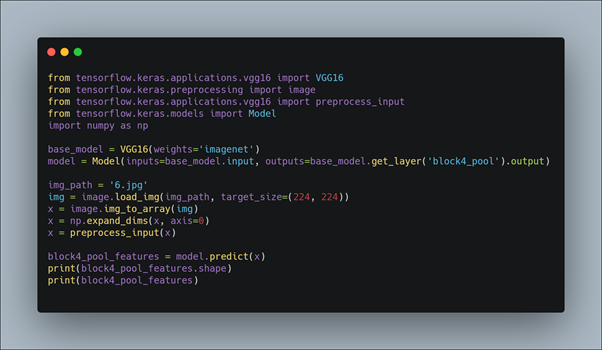
Here also we first import the VGG16 model from tensorflow keras. The image module is imported to preprocess the image object and the preprocess_input module is imported to scale pixel values appropriately for the VGG16 model. The numpy module is imported for array-processing. In addition the Model module is imported to design a new model that is a subset of the layers in the full VGG16 model. The model would have the same input layer as the original model, but the output would be the output of a given convolutional layer, which we know would be the activation of the layer or the feature map. Then the VGG16 model is loaded with the pretrained weights for the imagenet dataset. For example, after loading the VGG model, we can define a new model that outputs a feature map from the block4 pooling layer. After defining the model, we need to load the input image with the size expected by the model, in this case, 224×224. Next, the image PIL object needs to be converted to a NumPy array of pixel data and expanded from a 3D array to a 4D array with the dimensions of [samples, rows, cols, channels], where we only have one sample. The pixel values then need to be scaled appropriately for the VGG model. We are now ready to get the features.

For example here we extract features of block4_pool layer.

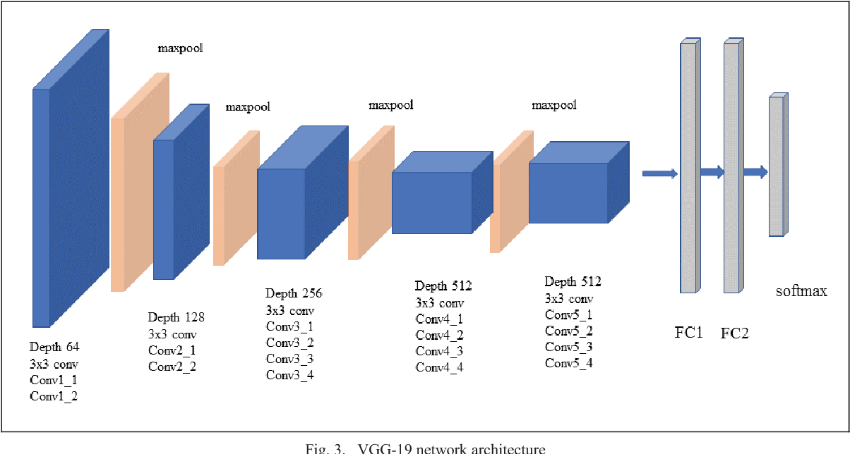
Extract features with VGG19

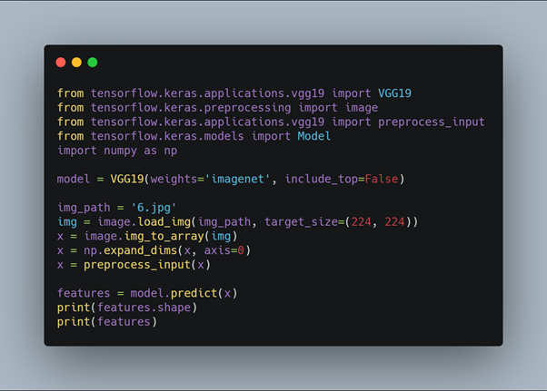
Here we first import the VGG19 model from tensorflow keras. The image module is imported to preprocess the image object and the preprocess_input module is imported to scale pixel values appropriately for the VGG19 model. The numpy module is imported for array-processing. Then the VGG19 model is loaded with the pretrained weights for the imagenet dataset. VGG19 model is a series of convolutional layers followed by one or a few dense (or fully connected) layers. Include_top lets you select if you want the final dense layers or not. False indicates that the final dense layers are excluded when loading the model. From the input layer to the last max pooling layer (labeled by 7 x 7 x 512) is regarded as feature extraction part of the model, while the rest of the network is regarded as classification part of the model. After defining the model, we need to load the input image with the size expected by the model, in this case, 224×224. Next, the image PIL object needs to be converted to a NumPy array of pixel data and expanded from a 3D array to a 4D array with the dimensions of [samples, rows, cols, channels], where we only have one sample. The pixel values then need to be scaled appropriately for the VGG model. We are now ready to get the features

Extract Features from an Arbitrary Intermediate Layer with VGG19

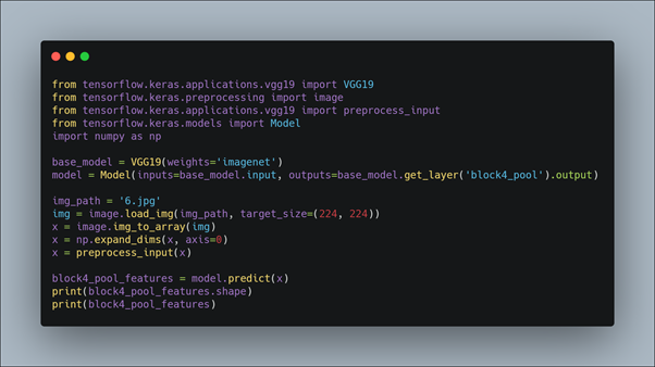
Here also we first import the VGG19 model from tensorflow keras. The image module is imported to preprocess the image object and the preprocess_input module is imported to scale pixel values appropriately for the VGG19 model. The numpy module is imported for array-processing. In addition the Model module is imported to design a new model that is a subset of the layers in the full VGG19 model. The model would have the same input layer as the original model, but the output would be the output of a given convolutional layer, which we know would be the activation of the layer or the feature map. Then the VGG19 model is loaded with the pretrained weights for the imagenet dataset. For example, after loading the VGG model, we can define a new model that outputs a feature map from the block4 pooling layer. After defining the model, we need to load the input image with the size expected by the model, in this case, 224×224. Next, the image PIL object needs to be converted to a NumPy array of pixel data and expanded from a 3D array to a 4D array with the dimensions of [samples, rows, cols, channels], where we only have one sample. The pixel values then need to be scaled appropriately for the VGG model. We are now ready to get the features.

For example here we extract features of block4_pool layer.

Summarize Filters in Each Convolutional Layer of VGG16 Model

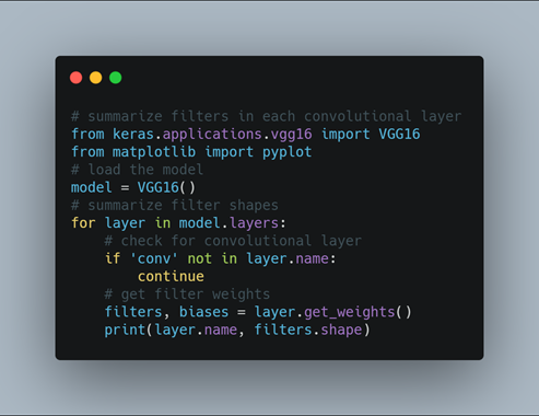
Filters are simply weights, yet because of the specialized two-dimensional structure of the filters, the weight values have a spatial relationship to each other and plotting each filter as a two-dimensional image is meaningful. Here we review the filters in the VGG16 model. Here we import the VGG19 model from tensorflow keras. We can access all of the layers of the model via the model.layers property. Each layer has a layer.name property, where the convolutional layers have a naming convolution like block#_conv#, where the ‘#‘ is an integer. Therefore, we can check the name of each layer and skip any that don’t contain the string ‘conv‘. Each convolutional layer has two sets of weights. One is the block of filters and the other is the block of bias values. These are accessible via the layer.get_weights() function. We can retrieve these weights and then summarize their shape. The complete example of summarizing the model filters is given above and the results are shown below.

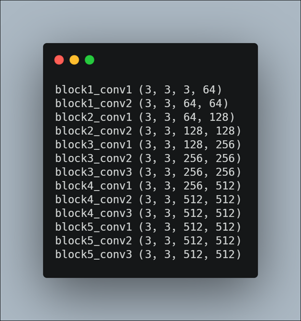
All convolutional layers use 3×3 filters, which are small and perhaps easy to interpret. An architectural concern with a convolutional neural network is that the depth of a filter must match the depth of the input for the filter (e.g. the number of channels). We can see that for the input image with three channels for red, green and blue, that each filter has a depth of three (here we are working with a channel-last format). We could visualize one filter as a plot with three images, one for each channel, or compress all three down to a single color image, or even just look at the first channel and assume the other channels will look the same.

Visualize First 6 Filters Out of 64 Filters in Second Layer of VGG16 Model

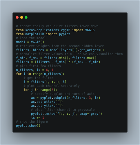
Here we retrieve weights from the second hidden layer of VGG16 model. The weight values will likely be small positive and negative values centered around 0.0. We can normalize their values to the range 0–1 to make them easy to visualize. We can enumerate the first six filters out of the 64 in the block and plot each of the three channels of each filter. We use the matplotlib library and plot each filter as a new row of subplots, and each filter channel or depth as a new column. Here we plot the first six filters from the first hidden convolutional layer in the VGG16 model.

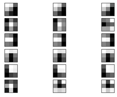
It creates a figure with six rows of three images, or 18 images, one row for each filter and one column for each channel. We can see that in some cases, the filter is the same across the channels (the first row), and in others, the filters differ (the last row). The dark squares indicate small or inhibitory weights and the light squares represent large weights. Using this intuition, we can see that the filters on the first row detect a gradient from light in the top left to dark in the bottom right.

Summarize Feature Map Size for Each Conv Layer

The activation maps, called feature maps, capture the result of applying the filters to input, such as the input image or another feature map. The idea of visualizing a feature map for a specific input image would be to understand what features of the input are detected or preserved in the feature maps. The expectation would be that the feature maps close to the input detect small or fine-grained detail, whereas feature maps close to the output of the model capture more general features. In order to explore the visualization of feature maps, we need input for the VGG16 model that can be used to create activations.

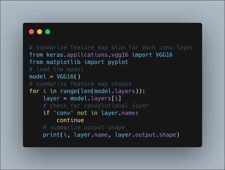
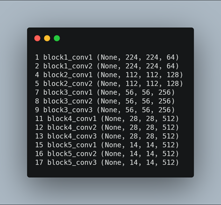
We need a clearer idea of the shape of the feature maps output by each of the convolutional layers and the layer index number. So we enumerate all layers in the model and print the output size or feature map size for each convolutional layer as well as the layer index in the model.

Visualizing the Feature Map for the First Convolutional Layer in the VGG16 Model for an Input Image

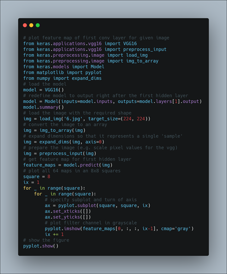
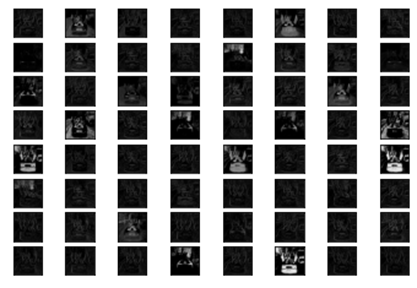
Here we design a new model that is a subset of the layers in the full VGG16 model. The model would have the same input layer as the original model, but the output would be the output of a given convolutional layer, which we know would be the activation of the layer or the feature map. After loading the VGG model, we can define a new model that outputs a feature map from the first convolutional layer. Making a prediction with this model will give the feature map for the first convolutional layer for a given provided input image. After defining the model, we need to load the input image with the size expected by the model, in this case, 224×224. Next, the image PIL object needs to be converted to a NumPy array of pixel data and expanded from a 3D array to a 4D array with the dimensions of [samples, rows, cols, channels], where we only have one sample. The pixel values then need to be scaled appropriately for the VGG model. We are now ready to get the feature map. We can do this easy by calling the model.predict() function and passing in the prepared single image. We know the result will be a feature map with 224x224x64. We can plot all 64 two-dimensional images as an 8×8 square of images.

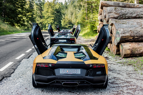
For a given image,

Visualize Feature Maps from the Five Main Blocks of the VGG16 Model

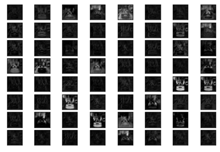
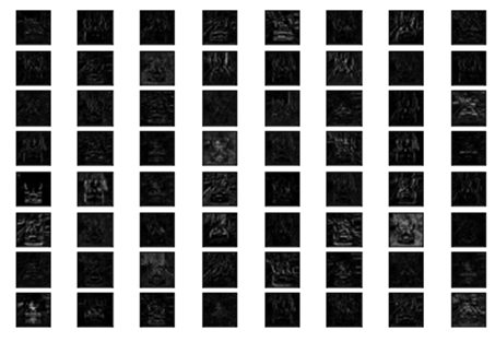
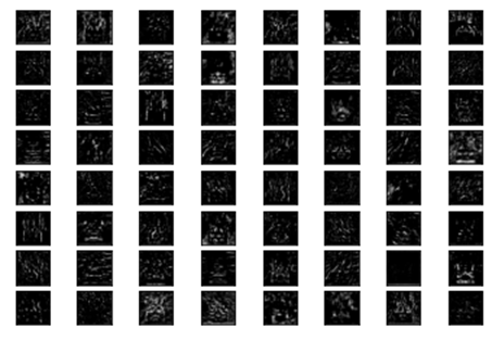
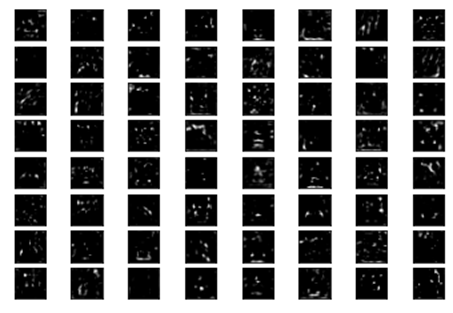
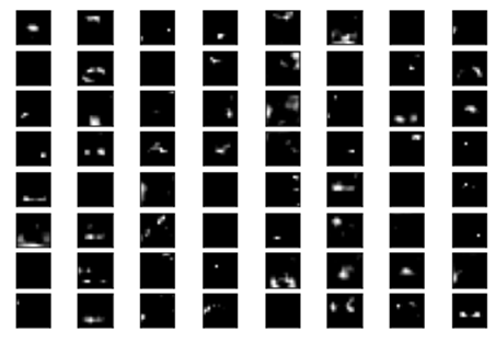
Here we collect feature maps output from each block of the model in a single pass, then create an image of each. There are five main blocks in the image (e.g. block1, block2, etc.) that end in a pooling layer. The layer indexes of the last convolutional layer in each block are [2, 5, 9, 13, 17]. We can define a new model that has multiple outputs, one feature map output for each of the last convolutional layer in each block. Making a prediction with this new model will result in a list of feature maps. We know that the number of feature maps (e.g. depth or number of channels) in deeper layers is much more than 64, such as 256 or 512. Nevertheless, we can cap the number of feature maps visualized at 64 for consistency. Here we create five separate plots for each of the five blocks in the VGG16 model for our input image.

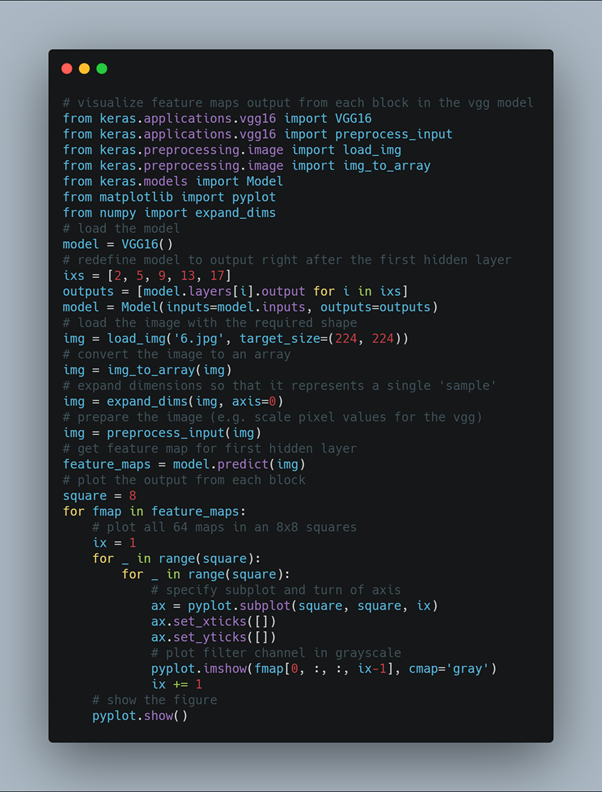
Running the example results in five plots showing the feature maps from the five main blocks of the VGG16 model. We can see that the feature maps closer to the input of the model capture a lot of fine detail in the image and that as we progress deeper into the model, the feature maps show less and less detail. This pattern was to be expected, as the model abstracts the features from the image into more general concepts that can be used to make a classification. Although it is not clear from the final image that the model saw a car, we generally lose the ability to interpret these deeper feature maps.

For a given image,

Hope you have gained some good knowledge about how to Extract Features, Visualize Filters and Feature Maps in VGG16 and VGG19 CNN Models. Stay tuned for more amazing articles.