Exploring the Efficacy and Applications of Modular Neural Networks in Modern AI

Introduction

In the rapidly evolving landscape of artificial intelligence, Modular Neural Networks (MNNs) have emerged as a pivotal innovation. Unlike traditional neural network architectures that follow a monolithic approach, MNNs employ a decentralized structure. This essay delves into the fundamentals of MNNs, their advantages, applications, and the challenges they pose.

In the realm of artificial intelligence, Modular Neural Networks stand as a testament to the power of collaborative intelligence, embodying the principle that the whole is greater than the sum of its parts.

Understanding Modular Neural Networks

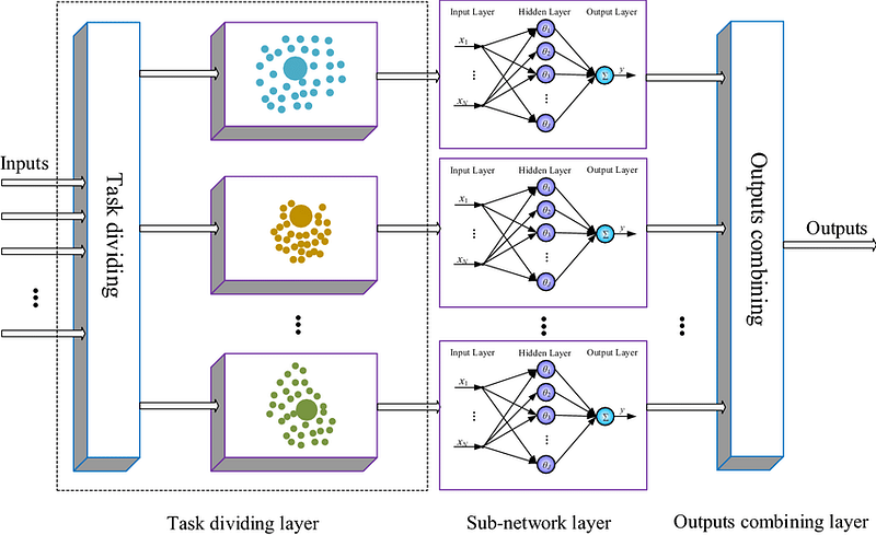
Modular Neural Networks represent a paradigm shift in neural network design. The core idea is to decompose a complex problem into smaller, manageable sub-tasks, each handled by a dedicated module. These modules are essentially individual neural networks trained to specialize in specific aspects of the overall task. The outputs of these modules are then integrated to formulate a comprehensive solution.

In MNNs, each module is trained separately, allowing for specialization. This decentralized training approach contrasts with traditional networks where a single model is trained on all aspects of a task. After training, these modules collaborate, either through a hierarchical structure or a network where the outputs of some modules serve as inputs for others.

Advantages of Modular Neural Networks

1. Specialization and Efficiency: The compartmentalized nature of MNNs allows for specialization, leading to increased efficiency and effectiveness in solving complex tasks. Each module becomes an expert in its specific domain, making the network adept at handling multifaceted problems.
2. Scalability and Flexibility: MNNs offer superior scalability and flexibility. New modules can be added or existing ones updated without retraining the entire network. This modular architecture makes MNNs particularly suitable for evolving tasks and environments.
3. Parallel Processing and Speed: The decentralized structure facilitates parallel processing, significantly speeding up computation. Since modules can operate independently, MNNs are well-suited for distributed computing environments.

Applications of Modular Neural Networks

1. Robotics and Autonomous Systems: In robotics, MNNs can control different parts or functions of a robot. For instance, separate modules could handle sensory processing, movement coordination, and decision-making, leading to more efficient and adaptable robotic systems.
2. Complex Problem Solving: MNNs excel in solving complex problems that can be broken down into smaller parts. This includes areas like natural language processing, where different modules can handle syntax, semantics, and context.
3. Personalization and Adaptive Systems: In recommendation systems and personalized content delivery, MNNs can adapt to individual user preferences and behaviors by adjusting specific modules without overhauling the entire system.

Challenges and Future Directions

1. Integration and Coordination: One of the primary challenges in MNNs is the integration and coordination of modules. Ensuring seamless communication and collaboration between modules is crucial for the effectiveness of the network.
2. Complexity in Design and Maintenance: Designing and maintaining MNNs can be complex. Determining the optimal number of modules, their specific roles, and the overall architecture requires careful planning and expertise.
3. Future Prospects: Future research in MNNs is likely to focus on automated module integration, advanced training algorithms for inter-module communication, and exploring applications in more diverse fields.

Code

Creating a complete code example for Modular Neural Networks (MNNs) in Python involves several steps: generating a synthetic dataset, designing individual modules for the network, training these modules, and finally integrating them. For demonstration purposes, I’ll create a simplified MNN that tackles a classification problem using a synthetic dataset. We’ll use libraries like numpy for data manipulation and tensorflow for building and training neural networks.

Make sure you have TensorFlow and other required libraries installed. You can install them using pip:

pip install numpy tensorflow matplotlib sklearn

Let’s begin by writing the Python code:

import numpy as np
import tensorflow as tf
from sklearn.datasets import make_classification
from sklearn.model_selection import train_test_split
from sklearn.metrics import accuracy_score
import matplotlib.pyplot as plt

# Step 2: Generate Synthetic Dataset
X, y = make_classification(n_samples=1000, n_features=20, n_informative=15, n_redundant=5, random_state=42)
X_train, X_test, y_train, y_test = train_test_split(X, y, test_size=0.2, random_state=42)

# Split features for two modules
X_train_mod1 = X_train[:, :10]
X_train_mod2 = X_train[:, 10:]
X_test_mod1 = X_test[:, :10]
X_test_mod2 = X_test[:, 10:]

# Step 3: Designing Modular Neural Networks
def create_module(input_shape):
    model = tf.keras.models.Sequential([
        tf.keras.layers.Dense(64, activation='relu', input_shape=input_shape),
        tf.keras.layers.Dense(32, activation='relu'),
        tf.keras.layers.Dense(16, activation='relu')
    ])
    return model

module1 = create_module((10,))
module2 = create_module((10,))

# Step 4: Training the Modules
module1.compile(optimizer='adam', loss='sparse_categorical_crossentropy', metrics=['accuracy'])
module2.compile(optimizer='adam', loss='sparse_categorical_crossentropy', metrics=['accuracy'])

module1.fit(X_train_mod1, y_train, epochs=10, batch_size=32, verbose=0)
module2.fit(X_train_mod2, y_train, epochs=10, batch_size=32, verbose=0)

# Step 5: Integration and Final Classification
combined_input = tf.keras.layers.concatenate([module1.output, module2.output])
final_output = tf.keras.layers.Dense(2, activation='softmax')(combined_input)
final_model = tf.keras.models.Model(inputs=[module1.input, module2.input], outputs=final_output)

final_model.compile(optimizer='adam', loss='sparse_categorical_crossentropy', metrics=['accuracy'])
final_model.fit([X_train_mod1, X_train_mod2], y_train, epochs=10, batch_size=32, verbose=0)

# Evaluation
y_pred = np.argmax(final_model.predict([X_test_mod1, X_test_mod2]), axis=1)
accuracy = accuracy_score(y_test, y_pred)
print(f'Accuracy: {accuracy}')

# Step 6: Plotting the Results
# Here you can add any specific plots you want, like loss curves or accuracy over epochs.
import matplotlib.pyplot as plt

# Modifying the training process to store history
history1 = module1.fit(X_train_mod1, y_train, epochs=10, batch_size=32, verbose=0, validation_split=0.2)
history2 = module2.fit(X_train_mod2, y_train, epochs=10, batch_size=32, verbose=0, validation_split=0.2)
final_history = final_model.fit([X_train_mod1, X_train_mod2], y_train, epochs=10, batch_size=32, verbose=0, validation_split=0.2)

# Plotting
plt.figure(figsize=(12, 6))

# Plot training & validation accuracy values for Module 1
plt.subplot(2, 3, 1)
plt.plot(history1.history['accuracy'])
plt.plot(history1.history['val_accuracy'])
plt.title('Module 1 Accuracy')
plt.ylabel('Accuracy')
plt.xlabel('Epoch')
plt.legend(['Train', 'Test'], loc='upper left')

# Plot training & validation loss values for Module 1
plt.subplot(2, 3, 2)
plt.plot(history1.history['loss'])
plt.plot(history1.history['val_loss'])
plt.title('Module 1 Loss')
plt.ylabel('Loss')
plt.xlabel('Epoch')
plt.legend(['Train', 'Test'], loc='upper left')

# Plot training & validation accuracy values for Module 2
plt.subplot(2, 3, 3)
plt.plot(history2.history['accuracy'])
plt.plot(history2.history['val_accuracy'])
plt.title('Module 2 Accuracy')
plt.ylabel('Accuracy')
plt.xlabel('Epoch')
plt.legend(['Train', 'Test'], loc='upper left')

# Plot training & validation loss values for Module 2
plt.subplot(2, 3, 4)
plt.plot(history2.history['loss'])
plt.plot(history2.history['val_loss'])
plt.title('Module 2 Loss')
plt.ylabel('Loss')
plt.xlabel('Epoch')
plt.legend(['Train', 'Test'], loc='upper left')

# Plot training & validation accuracy values for Final Model
plt.subplot(2, 3, 5)
plt.plot(final_history.history['accuracy'])
plt.plot(final_history.history['val_accuracy'])
plt.title('Final Model Accuracy')
plt.ylabel('Accuracy')
plt.xlabel('Epoch')
plt.legend(['Train', 'Test'], loc='upper left')

# Plot training & validation loss values for Final Model
plt.subplot(2, 3, 6)
plt.plot(final_history.history['loss'])
plt.plot(final_history.history['val_loss'])
plt.title('Final Model Loss')
plt.ylabel('Loss')
plt.xlabel('Epoch')
plt.legend(['Train', 'Test'], loc='upper left')

plt.tight_layout()
plt.show()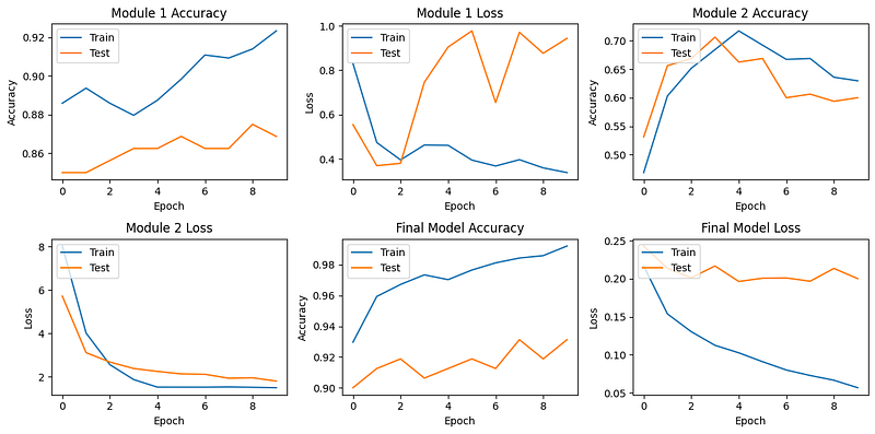

This script demonstrates a basic implementation of a Modular Neural Network. Depending on your specific problem, the architecture, number of modules, and the way they’re integrated might vary significantly. Also, remember to adjust the epochs, batch size, and network layers according to the complexity of your task.

Conclusion

Modular Neural Networks mark a significant advancement in the field of AI, offering a flexible, efficient, and scalable approach to problem-solving. Their ability to handle complex, multifaceted tasks makes them a valuable tool in various applications. While they present certain challenges, ongoing research and development promise to further enhance their capabilities, solidifying their role in the future of artificial intelligence.