Exploring Behavioral Finance Models in Algorithmic Trading

Behavioral finance is a fascinating field that combines psychology and finance to understand how human behavior influences financial markets. In algorithmic trading, exploiting human cognitive biases can lead to the development of quantitative strategies that outperform traditional approaches. In this tutorial, we will explore the application of behavioral finance models in algorithmic trading using Python.

We will leverage the yfinance library to download financial data for a diverse set of securities listed on Yahoo Finance. By analyzing this data and incorporating behavioral finance concepts, we will develop quantitative trading strategies that take advantage of common cognitive biases exhibited by market participants.

Setting Up the Environment

Before we begin, let’s ensure we have all the necessary libraries installed. We will start by installing the yfinance library to download financial data.

pip install yfinance

Next, let’s import the required libraries in our Python script.

import yfinance as yf
import numpy as np
import matplotlib.pyplot as plt
import mplfinance as mpf

Downloading Financial Data

To demonstrate the application of behavioral finance models in algorithmic trading, we need historical financial data for our analysis. We will download data for a diverse set of securities until the end of February 2024.

# Downloading financial data for multiple securities
securities = ['GOOG', 'TSLA', 'NFLX', 'BTC-USD']  # Google, Tesla, Netflix, Bitcoin
start_date = '2020-01-01'
end_date = '2024-02-29'

data = {}
for security in securities:
    data[security] = yf.download(security, start=start_date, end=end_date)

Exploring Behavioral Finance Models

1. Loss Aversion

Loss aversion is a common cognitive bias where individuals prefer avoiding losses over acquiring equivalent gains. Let’s visualize the historical prices of Google stock (GOOG) and identify potential opportunities based on loss aversion.

# Visualizing historical prices of Google stock
mpf.plot(data['GOOG'], type='candle', volume=True, )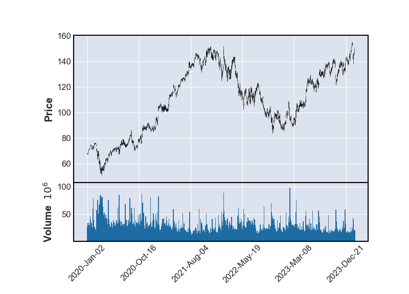

By analyzing the historical prices of Google stock, we can identify patterns that align with the concept of loss aversion. This information can be used to develop trading strategies that capitalize on market participants’ tendency to avoid losses.

2. Herding Behavior

Herding behavior refers to the tendency of individuals to follow the actions of a larger group, often leading to market inefficiencies. Let’s analyze the price movements of Tesla stock (TSLA) to identify instances of herding behavior.

# Visualizing historical prices of Tesla stock
mpf.plot(data['TSLA'], type='candle', volume=True, )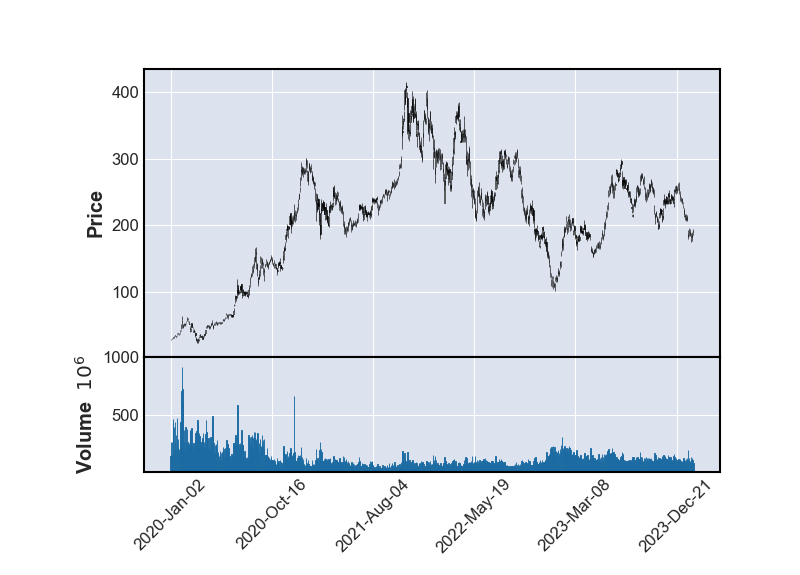

By studying the price movements of Tesla stock, we can uncover potential opportunities resulting from herding behavior in the market. This insight can be leveraged to develop trading strategies that exploit these inefficiencies.

Building Quantitative Trading Strategies

Now that we have explored behavioral finance models in the context of algorithmic trading, let’s develop quantitative trading strategies based on the insights gained from our analysis.

Strategy 1: Momentum Trading

Momentum trading is a popular strategy that involves buying securities that have exhibited upward price momentum and selling those that have shown downward momentum. Let’s implement a simple momentum trading strategy using the historical price data of Netflix stock (NFLX).

# Calculating 50-day and 200-day moving averages for Netflix stock
data['NFLX']['MA50'] = data['NFLX']['Close'].rolling(window=50).mean()
data['NFLX']['MA200'] = data['NFLX']['Close'].rolling(window=200).mean()

# Generating buy/sell signals based on moving average crossovers
data['NFLX']['Signal'] = np.where(data['NFLX']['MA50'] > data['NFLX']['MA200'], 1, 0)

# Plotting the trading signals
plt.figure(figsize=(14, 7))
plt.plot(data['NFLX']['Close'], label='NFLX Close Price', alpha=0.7)
plt.plot(data['NFLX']['MA50'], label='50-day MA', alpha=0.7)
plt.plot(data['NFLX']['MA200'], label='200-day MA', alpha=0.7)
plt.plot(data['NFLX'][data['NFLX']['Signal'] == 1].index, 
         data['NFLX']['MA50'][data['NFLX']['Signal'] == 1], '^', markersize=10, color='g', lw=0, label='Buy Signal')
plt.plot(data['NFLX'][data['NFLX']['Signal'] == 0].index, 
         data['NFLX']['MA50'][data['NFLX']['Signal'] == 0], 'v', markersize=10, color='r', lw=0, label='Sell Signal')
plt.title('Netflix Stock - Momentum Trading Strategy')
plt.legend()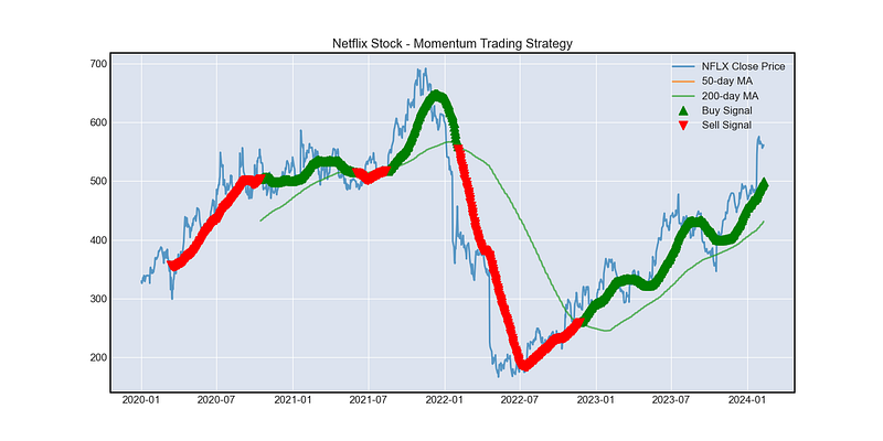

In this strategy, we generate buy signals when the 50-day moving average crosses above the 200-day moving average and sell signals when the opposite occurs. By implementing this momentum trading strategy, we aim to capitalize on trends in Netflix stock prices.

Conclusion

In this tutorial, we have explored the application of behavioral finance models in algorithmic trading using Python. By leveraging historical financial data and behavioral insights, we developed quantitative trading strategies that exploit common cognitive biases exhibited by market participants.

Understanding human behavior and its impact on financial markets is crucial for building robust trading strategies. By incorporating behavioral finance concepts into algorithmic trading, we can enhance our decision-making processes and potentially achieve better trading outcomes.

As you continue to explore the intersection of behavioral finance and algorithmic trading, remember to test and refine your strategies based on real-world data and market conditions. Stay curious, keep learning and enjoy the journey of building sophisticated trading models with Python!