Explore the Power of the Central Limit Theorem for A/B Testing

In previous articles, we discussed how to calculate sample size using power analysis and explored concepts such as confidence intervals and statistical significance. Now, let’s dive into the Central Limit Theorem and understand its impotance when conducting statistical analysis, and A/B tests.

Imagine you want to find out the average height of all 10-year-old kids in your city. The first thing you may consider is to measure every single kid in the city, but that would be impractical and time-consuming. Instead, you decide to randomly select a group of kids and measure their heights. However, if you were to measure just ten kids, those few measurements might not accurately represent the entire population’s average height since they could include unusually tall or short children.

To find the average height of all kids, suppose, you take a random sample of at least 50 kids, and this sample has to be truly random. Then you measure all kids in your sample and calculate the average height of this sample. Then you collect many such random samples, suppose 100 samples with 50 kids height each, and again calculate the average height for each. After all the calculations you plot all averages of all samples.

What you will notice is that the distribution of the averages will look like a bell-shaped curve — normal distribution. The more random samples you calculate the average the more clearly you will see the effect of the central limit theorem, which stands that as the number of sample increases, the distribution of sample means tends to approximate a normal distribution, regardless of the shape of the population distribution. In other words, even if the individual heights of the kids in the city are not normally distributed, the distribution of the sample means will tend to be normal.

By following the central limit theorem, you can have confidence that by measuring more kids’ heights and calculating their average, you will obtain a more accurate estimation of the average height of all 10-year-old kids in the city. The central limit theorem helps statisticians and researchers make better predictions and understand how data behaves.

Another good example of the central limit theorem is the Galton Board. This device, invented by Sir Francis Galton, was designed to demonstrate the central limit theorem, specifically showing that with a sufficient sample size, the binomial distribution approximates a normal distribution.

The Galton Board is a simple device used to illustrate probability and the concept of the normal distribution. It consists of a board with pegs arranged in a triangular pattern. When you drop a ball from the top, it randomly bounces off the pegs and eventually falls into slots at the bottom. As more and more balls are dropped, they tend to accumulate in a pattern that follow a bell-shaped curve, which is known as the normal distribution. The Galton Board helps us visualize how random events can follow a predictable pattern, and it is often used as a tool for teaching about probability and statistics.

Step by Step — Central Limit Theorem

Let’s explore an step-by-step example to illustrate the central limit theorem.

Suppose you want to determine the average height of all 10-year-old kids in a city. Step 1: you choose to take one sample of 50 children and measure their heights. After randomly measuring 50 kids, you obtain the following heights:

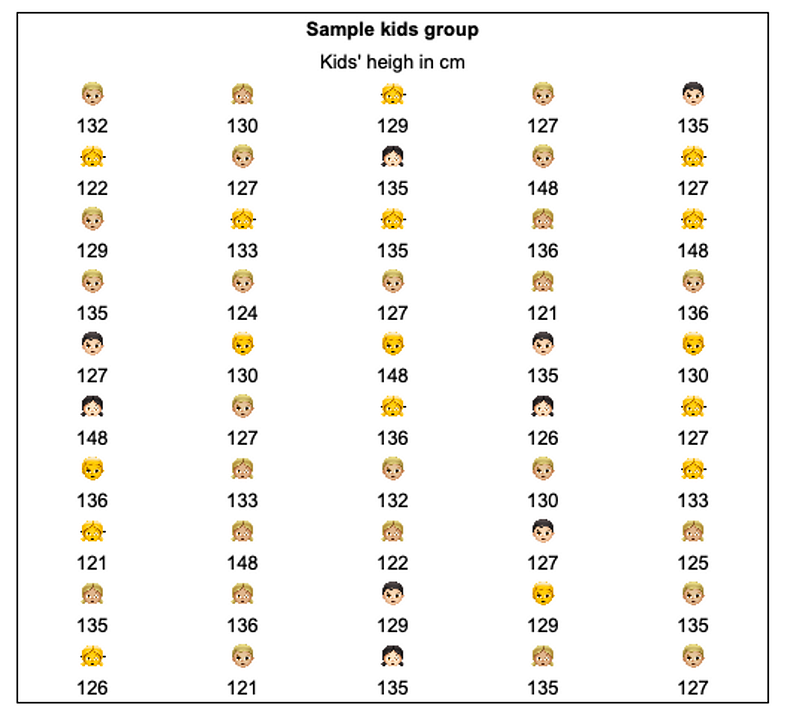
Step 2: Calculate the mean (average) of the heights in the sample:

To calculate the mean, sum up all the heights in the sample and divide by the total number of measurements.

Mean = (132 + 122 + 129 + … + 125 + 135 + 127) / 50 = 131.7 cm.

The mean of this sample is 131.7 centimeters.

Step 3: Repeat Steps 1 and 2 for n-number of times to collect multiple random samples and calculate their means. (For the purpose of this example, let’s consider using 50 random samples of the heights of 50 kids to illustrate the distribution of the means.)

Step 4: Plot all the sample means and observe the distribution.

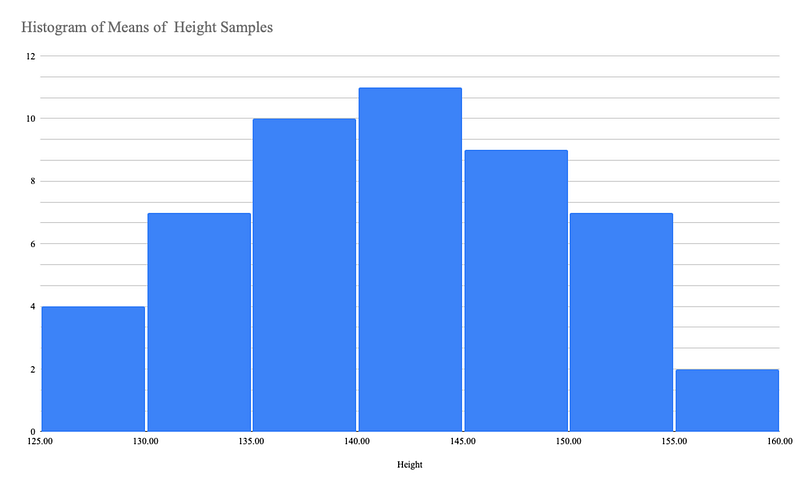
By performing Steps 1 and 2 for multiple random samples, you can calculate the mean height for each sample. After collecting these means from different samples, you can plot them and observe their distribution. As we can see the distribution is likely to follow a bell-shaped curve, indicating the central limit theorem in action. The more samples you include, the clearer the bell-shaped distribution becomes, demonstrating the approximation to a normal distribution.

Step 5: Make conclusions. Based on the central limit theorem, we can conclude that the distribution of the sample means tends to approach a normal distribution, irrespective of the shape of the population distribution. This allows us to make inferences about the population parameter, such as the average heights of all 10-year-old kids in the city, utilizing the properties of the normal distribution.

Use central limit theorem to make inferences

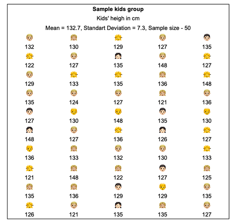
Let’s consider the same scenario of estimating the average height of 10-year-old kids in the city, but this time we use Central Limit Theorem to make inferences. We randomly choose 50 10 year old kids in the city and calculate the average height in this sample

For example: Average height = (132 + 122 + 129 + … + 125 + 135 + 127) / 50 = 131.7 cm.

The average height of this sample turns out to be 131.7 centimeters.

Next, you can utilize the central limit theorem to make inferences about the population, as based on the central limit theorem we can assume that the distribution of sample means approximates a normal distribution. By leveraging the properties of the normal distribution, you estimate the range within which the true population mean is likely to fall. One way to achieve this is by calculating a confidence interval, which provides a range of values that is expected to contain the true population mean with a specified level of confidence.

To calculate a confidence interval, you need three pieces of information: the desired confidence level, the standard deviation (or an estimate of it), and the sample size. In case you want to learn more, we have covered how to calculate confidence interval in Understanding Confidence Intervals in A/B Testing: Exploring the Range of Effect Sizes and Statistical Significance article.

Let’s say you calculate a 95% confidence interval for the average height of 10-year-old kids in the city, and the sample size is 50. In many cases, we do not have knowledge of the population standard deviation, so we rely on the sample standard deviation as an estimate to calculate the confidence interval. This is a common approach in statistics when dealing with real-life data.

Additionally, as the sample size increases, the sample standard deviation becomes a more reliable estimate of the population standard deviation, and the confidence interval becomes narrower and more precise.

Confidence Interval = Sample Mean ± Margin of Error.

• Where the Margin of Error = (Z * (Population Standard Deviation / √Sample Size)), and the standard deviation is 7.3.
• Note: Z is the critical value from the standard normal distribution corresponding to the desired confidence level. For a 95% confidence level, Z is approximately 1.96.

By performing the calculations, we find that the Margin of Error is 2.04. The next step is to determine the lower and upper limits of the confidence interval:

• Lower = Sample Mean — Margin of Error, 131.7–2.04 = 129.66 cm
• Upper = Sample Mean + Margin of Error, 131.7 + 2.04 = 133.74 cm

This implies that the 95% confidence interval for the average height of all 10-year-old children in the city is approximately between 129.66 centimeters to 133.74 centimeters.

Consequently, we can state with 95% confidence that the true average height of all 10-year-old children in the city falls within this range, based on our sample.

The central limit theorem is a fundamental concept in statistics and probability theory. Here are a few examples what it enables us to do:

1. In A/B Testing, or hypothesis testing the theorem allows us to make inferences about population. When conducting the hypothesis tests, the theorem helps in determining the critical values and calculating p-values. It allows us to approximate the sampling distribution of test statistics, such as the t-statistic or the z-score, under the null hypothesis.
2. In Power Analysis, it helps us to determine the sample size required to detect a specific effect size with a given level of statistical power.
3. In Confidence Intervals, we use the theorem to construct the confidence intervals for population parameters.

Overall, the central limit theorem is a fundamental tool that enables statisticians, researchers, and professionals in various fields to make reliable inferences, estimate parameters, and understand the behavior of data distributions.

Want to learn data science? Here is the complete end-to-end data science project for beginners to learn data science. By completing this project: 1) you will experience the entire data science cycle yourself, 2) you will develop a project that you can use to prove your experience, and 3) you will answer the most popular interview questions in case you decide to pursue the career of a data scientist. You can find it on Amazon:

What do you struggle with in your early journey? Please share it with me here, and I am happy to help! I listen to your stories carefully and want to produce content that helps you in this journey. For more content like this, sign up for my newsletter.