Expectation-Maximization

The expectation-maximization (EM) algorithm is a powerful iterative method for estimating the parameters of statistical models, in cases where their equations cannot be solved directly. Typically, these models contain latent (hidden) variables in addition to the unknown parameters of the probability distributions.

The EM algorithm is used in various machine learning applications, such as speech recognition, image classification, and NLP (natural language processing).

This article is a bit math-heavy, so buckle up :) I promise to make the definitions and mathematical notations as clear as possible. If you are not familiar with the concept of maximum likelihood, I recommend that you first read my previous article on this topic.

Mixture Models

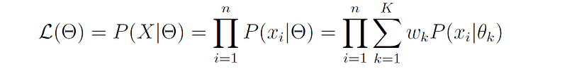
EM is frequently used for parameter estimation of mixture models. A mixture model assumes that the data is generated from a collection of probability distributions D₁, …, Dₖ with mixing weights or proportions w₁, …, wₖ, where k is the number of distributions and the weights sum to 1.

The probability distribution of the mixture model can be written as:

where P(x|Dⱼ) is the probability density function (PDF) of distribution j.

One of the most common mixture models is called GMM (Gaussian Mixture Model), where the distributions D₁, …, Dₖ are assumed to be Gaussian (normal) distributions, i.e.,

Note that each distribution in the mixture has its own mean and standard deviation parameters, denoted by μⱼ and σⱼ respectively.

GMMs are used in a variety of machine learning applications, e.g., for clustering and density estimation.

Typically, both the distributions’ parameters (e.g., the μⱼ and σⱼ in GMMs) and the weights of the distributions (wⱼ) are unknown, and we would like to infer them from our data points.

Maximum Likelihood of Mixture Models

Assume that we have a set of n data points denoted by X = {x₁, x₂, … , xₙ}, that are generated from our mixture model. Let’s denote the parameters of the distributions in the mixture model by θ₁, …, θₖ, and the overall set of model parameters (including the weights) by Θ.

We would like to find the parameters Θ of the model that maximizes the likelihood of the data X, which can be written as:

The typical procedure in MLE (maximum likelihood estimation) is to take the derivatives of the log likelihood with respect to each parameter of the model and set it to zero. However, in the case of mixture models, the system of equations that we get is non-linear and therefore cannot be solved directly.

Instead, we can use the EM algorithm to find the set of parameters Θ that best fits our data.

The EM algorithm

1. Select an initial set of model parameters (e.g., by picking them randomly from some range).
2. Expectation step (E-step): For each data point xᵢ, compute the probability that it belongs to each distribution.
3. Maximization step (M-step): Given the probabilities from the E-step, find the new estimates of the model parameters that maximize the expected likelihood of the model.
4. Repeat steps 2 and 3 until the model parameters do not change (or stop when the change in the log-likelihood or the parameter estimates falls below a specified threshold).

Let’s dive deeper into the implementation details of each step in the algorithm.

In the E-step, we need to compute for each data point xᵢ and each class j, the probability that xᵢ belongs to class j, or P(dᵢ = j|xᵢ, Θ) (dᵢ is a variable that represents the distribution that point xᵢ belongs to). To compute this probability, we can use Bayes’ rule:

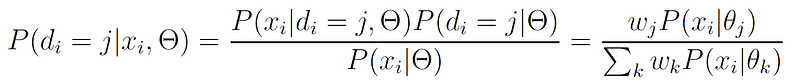
The probabilities P(xᵢ|θⱼ) are just the probability density functions of our distributions (e.g., normal distributions in the case of GMMs).

In the M-step, we update the parameters of our model.

First, we update the weights of the distributions:

The new weight of each distribution is given by the total probability of all the points belonging to that distribution, normalized by the number of points n.

Next, we update the parameters of the distributions themselves. In the case of GMMs, this means updating the mean μⱼ and standard deviation σⱼ of each distribution. As we have shown in my previous article, the MLE for the parameters of a normal distribution are just the sample mean and standard deviation of the data points.

Therefore, the parameters of the normal distributions are updated using the following equations:

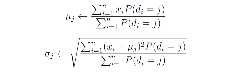
That is, the new mean (or standard deviation) of each distribution is the weighted mean (or standard deviation) of all the points that belong to that distribution (we multiply each point xᵢ by the probability that belongs to distribution j, and normalize by the total probabilities of all the points belonging to this distribution).