
Every Pandas Function You Can (Should) Use to Manipulate Time Series
From basic time-series metrics to window functions

Introduction to this project on Time Series Forecasting
Recently, the Optiver Realized Volatility Prediction competition has been launched on Kaggle. As the name suggests, it is a time series forecasting challenge.
I wanted to participate, but it turns out my knowledge in time series couldn’t even begin to suffice to participate in a competition of such a magnitude. So, I accepted this as the ‘kick in the pants’ I needed to start paying serious attention to this large sphere of ML.
As the first step, I wanted to learn and teach every single Pandas function you can use to manipulate time-series data. These functions are the basic requirements for dealing with any time series data you encounter in the wild.
I have got rather cool and interesting articles planned on this topic, and today, you will be reading the first taste of what is to come. Enjoy!
Table of Contents
The notebook of this article can be read here on Kaggle.
- Basic data and time functions
- Missing data imputation/interpolation in time series
- Basic time series calculations and metrics
- Resampling — upsample and downsample
- Comparing the growth of multiple time series
- Window functions
- Summary
1. Basic date and time functions in Pandas
1.1 Importing time-series data
When using the pd.read_csv function to import time series, there are 2 arguments you should always use - parse_dates and index_col:
The datasets have been anonymized due to publication policies. The real versions of the datasets are preserved in the notebook if you are interested. Note that this anonymity won’t hinder your experience.


parse_dates converts date-like strings to DateTime objects and index_col sets the passed column as the index. This operation is the basis for all time-series manipulation you will do with Pandas.
When you don’t know which column contains dates upon importing, you can perform the date conversion using pd.to_datetime function afterward:
Now, inspect the datetime format string:
>>> data2.head()
It is in the format “%Y-%m-%d” (full list of datetime format strings can be found here). Pass this to pd.to_datetime:
Passing a format string to pd.to_datetime significantly speeds up the conversion for large datasets. Set errors to "coerce" to mark invalid dates as NaT (not a date, i.e. - missing).
After conversion, set the DateTime column as index (a strict requirement for best time series analysis):
>>> data2.set_index("date", inplace=True)1.2 Pandas TimeStamp
The basic date data structure in Pandas is a timestamp:
You can make even more granular timestamps using the right format or, better yet, using the datetime module:
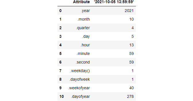
A full timestamp has useful attributes such as these:
1.3 Sequence of dates (timestamps)
A DateTime column/index in pandas is represented as a series of TimeStamp objects.
pd.date_range returns a special DateTimeIndex object that is a collection of TimeStamps with a custom frequency over a given range:
After specifying the date range (from October 10, 2010, to the same date in 2020), we are telling pandas to generate TimeStamps on a monthly-basis with freq='M':
>>> index[0]Timestamp('2010-10-31 00:00:00', freq='M')Another way to create date ranges is passing the start date and telling how many periods you want, and specifying the frequency:
Since we set the frequency to years, date_range with 5 periods returns 5 years/timestamp objects. The list of frequency aliases that can be passed to freq is large, so I will only mention the most important ones here:
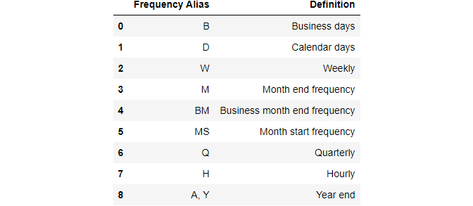
It is also possible to pass custom frequencies such as “1h30min”, “5D”, “2W”, etc. Again, check out this link for the full info.
1.4 Slicing
Slicing time series data can be very intuitive if the index is a DateTimeIndex. You can use something called partial slicing:


You can even go down to hours, minutes, or seconds levels if the DateTime is granular enough.
Note that pandas slices dates in closed intervals. For example, using “2010”: “2013” returns rows for all 4 years — it does not exclude the end of the period like integer slicing.
This date slicing logic applies to other operations like choosing a specific column after the slice:
2. Missing data imputation or interpolation
Missing data is ubiquitous no matter the type of the dataset. This section is all about imputing it in the context of time series.
You may also hear it called interpolation of missing data in time series lingo.
Besides the basic mean, median and mode imputation, some of the most common techniques include:
- Forward filling
- Backward filling
- Intermediate imputations with
pd.interpolate
We will also discuss model-based imputation such as KNN imputing. Moreover, we will explore visual methods of comparing the efficiency of the techniques and choose the one that best fits the underlying distribution.
2.1 Mean, median and mode imputation
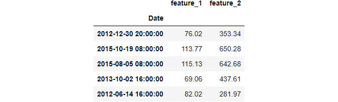
Let’s start with the basics. We will randomly select data points in the first anonymized dataset and convert them to NaN:
We will also create a function that plots the original distribution before and after an imputation(s) is performed:
We will start trying out techniques with SimpleImputer from Sklearn:
Let’s plot the original feature_2 distribution against the 3 imputed features we just created:
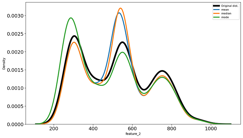
It is hard to say which lines most closely resembles the black line, but I will go with the green.
2.2 Forward and backward filling
Consider this small distribution:
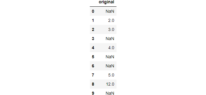
We will use both forward and backward filling and assign them back to the DataFrame as separate columns:
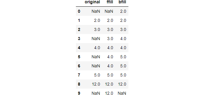
It should be fairly obvious how these methods work once you examine the above output.
Now, let’s perform these methods on the Airquality in India dataset:
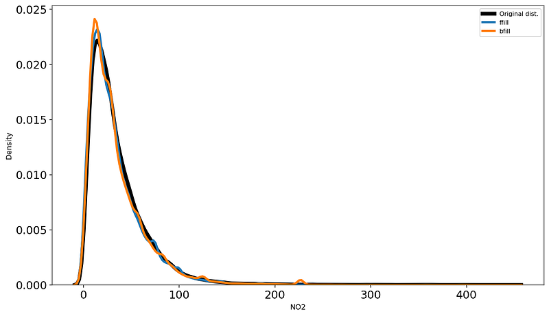
Even though very basic, forward and backward filling actually works pretty well on climate and stocks data since the differences between nearby data points are small.
2.3 Using pd.interpolate
Pandas provides a whole suite of other statistical imputation techniques in pd.interpolate function. Its method parameter accepts the name of the technique as a string.
The most popular ones are ‘linear’ and ‘nearest,’ but you can see the full list from the function’s documentation. Here, we will only discuss those two.
Consider this small distribution:

Once again, we apply the methods and assign their results back:
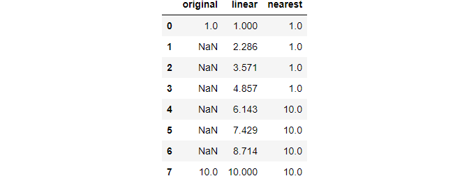
Neat, huh? The linear method considers the distance between any two non-missing points as linearly spaced and finds a linear line that connects them (like np.linspace). 'Nearest' method should be understandable from its name and the above output.
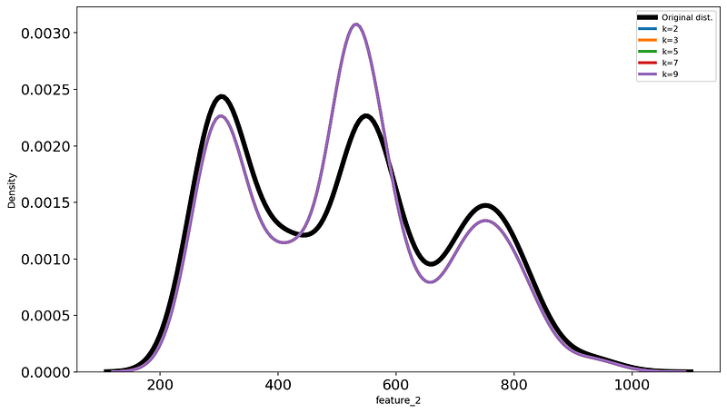
2.4 Model-based imputation with KNN
The last method we will see is the K-Nearest-Neighbors algorithm. I won’t detail how the algorithm works but only show how you can use it with Sklearn. If you want the details, I have a separate article here.
The most important parameter of KNN is k - the number of neighbors. We will apply the technique to the first dataset with several values of k and find the best one the same way as we did in the previous sections:
3. Basic time series calculations
Pandas offers basic functions to calculate the most common time series calculations. These are called shifts, lags, and something called a percentage change.
3.1 Shifts and lags
A common operation in time series is to move all data points one or more periods backward or forward to compare past and future values. You can do these operations using shift function of pandas. Let's see how to move the data points 1 and 2 periods into the future:
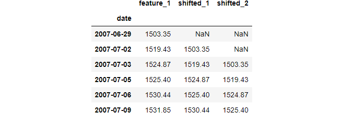
Shifting forward enables you to compare the current data point to those recorded one or more periods before.
You can also shift backward. This operation is also called “lagging”:
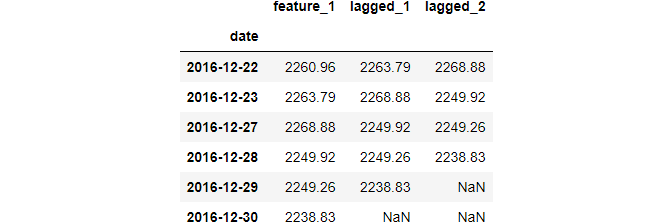
Shifting backward enables us to see the difference between the current data point and the one that comes one or more periods later.
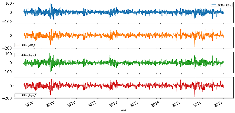
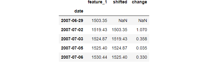
A common operation after shifting or lagging is finding the difference and plotting it:
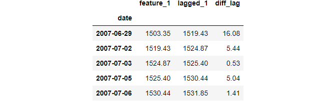
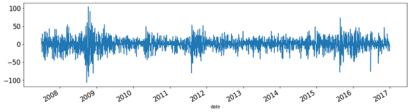
Since this operation is so common, Pandas has the diff function that computes the differences based on the period:
3.2 Percentage changes
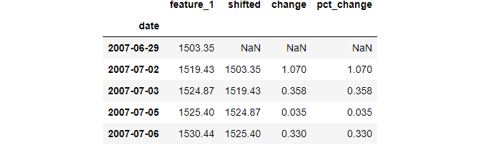
Another common metric that can be derived from time-series data is day-to-day percentage change:
To calculate day-to-day percentage change, shift one period forward and divide the original distribution by the shifted one and subtract 1. The resulting values are given as proportions of what they were the day before.
Since it is a common operation, Pandas implements it with the pct_change function:
4. Resampling
Often, you may want to increase or decrease the granularity of time series to generate new insights. These operations are called resampling or changing the frequency of time series, and we will discuss the Pandas functions related to them in this section.
4.1 Changing the frequency with asfreq
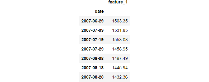
The second dataset does not have a fixed date frequency, i.e., the period difference between each date is not the same:
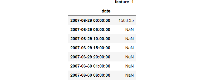
data2.head()Let’s fix this by giving it a calendar day frequency (daily):
data2.asfreq("D").head(7)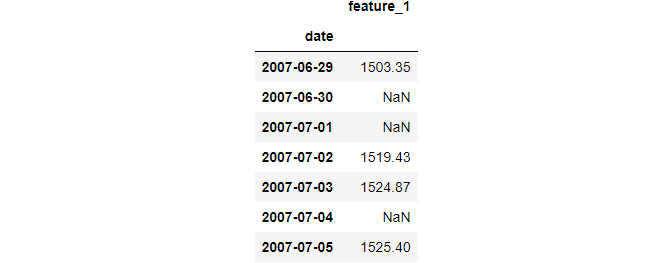
We just made the frequency of the date more granular. As a result, new dates were added, leading to more missing values. You can now interpolate them using any of the techniques we discussed earlier.
You can see the list of built-in frequency aliases from here. A more interesting scenario would be using custom frequencies:
# 10 month frequency
data2.asfreq("10M", method="bfill").head(7)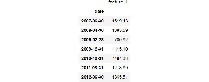
There is also a reindex function that operates similarly and supports additional missing value filling logic. We won't discuss it here as there are better options we will consider.
4.2 Downsampling with resample and aggregating
In time series lingo, making the frequency of a DateTime less granular is called downsampling. The examples are changing the frequency from hourly to daily, from daily to weekly, etc.
We saw how to downsample with asfreq. A more powerful alternative is resample which behaves like pd.groupby. Just like groupby groups the data based on categorical values, resample groups the data by date frequencies.
Let’s downsample the first dataset by month-end frequency:
Unlike asfreq, using resample only returns the data in the resampled state. To see each group, we need to use some type of function, similar to how we use groupby.
Since downsampling decreases the number of data points, we need an aggregation function like mean, median, or mode:
data1.resample("M").mean().tail()
There are also functions that return the first or last record of a group:


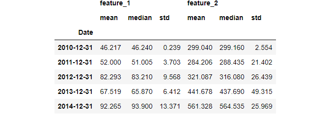
It is also possible to use multiple aggregating functions using agg:
4.3 Upsampling with resample and interpolating
The opposite of downsampling is making the DateTime more granular. This is called upsampling and includes operations like changing the frequency from daily to hourly, hourly to seconds, etc.
When upsampling, you introduce new dates leading to more missing values. This means you need to use some type of imputation:

4.4 Plotting the resampled data
Resampling isn’t going to give much if you don’t plot its results.
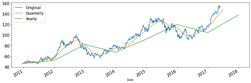
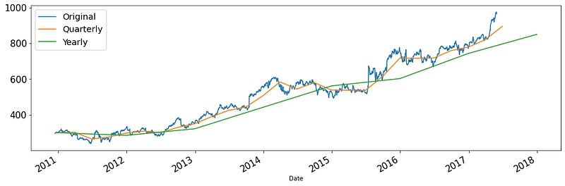
In most cases, you will see new trends and patterns when you downsample. This is because downsampling reduces the granularity, thus eliminating noise:
Plotting the upsampled distribution is only going to introduce more noise, so we won’t do it here.
5. Comparing the growth of multiple time series
It is common to compare two or more numeric values that change over time. For example, we might want to see the growth rate of feature 1 and 2 in the first dataset. But here is the problem:
The second distribution have much higher values. Plotting them together would probably squish feature_1 to a flat line. In other words, the two distributions have different scales.
To fix this, statisticians use normalization. The most common variation is choosing the first recorded value and dividing the rest of the samples by that amount. This shows how each record changes compared to the first.
Here is an example:
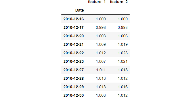
Each row in the above output now shows the percentage growth compared to the first row.
Now, let’s plot them to compare the growth rate:
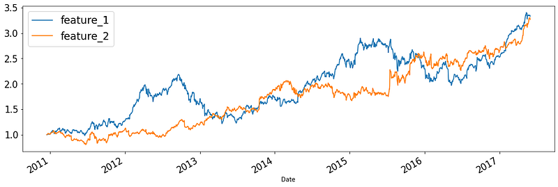
Both features achieved over 300% growth from 2011 to 2017. You can even plot time series from other datasets:
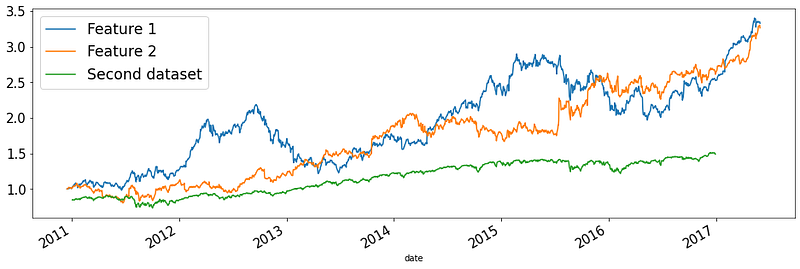
As you can see, features in dataset 1 have much higher growth than another feature in the second dataset.
6. Window functions
There is another type of function that helps you analyze time-series data in novel ways. These are called window functions, and they help you aggregate over a custom number of rows called ‘windows.’
For example, I can create a 30-day window over my Medium subscribers data to see the total number of subscribers for the past 30 days on any given day. Or a restaurant owner might create a weekly window to see average sales of the past week. Examples are endless as you can create a window of any size over your data.
Let’s explore these in more detail.
6.1 Rolling window functions
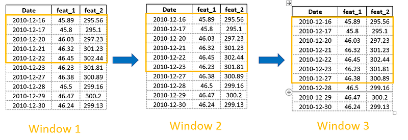
Rolling window functions will have the same length. As they slide through the data, their coverage (number of rows don’t change). Here is an example window of 5 periods sliding through the data:
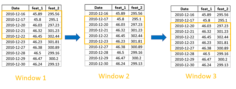
Here is how we create rolling windows in pandas:
>>> data1.rolling(window=5)Rolling [window=5,center=False,axis=0]Just like resample, it is in a read-only state - to use each window, we should chain some type of function. For example, let's create a cumulative sum for every past 5 periods:
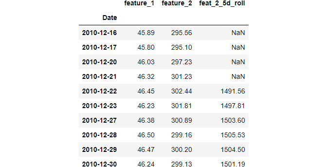
Obviously, the first 4 rows will be NaNs. Any other row will contain the sum of the previous 4 rows and the current one.
Pay attention to the window argument. If you pass an integer, the window size will be determined by that number of rows. If you pass a frequency alias such as months, years, 5 hours, or 7 weeks, the window size will be whatever number of rows that includes the single unit of the passed frequency. In other words, a 5-period window might have a different size than a 5-day frequency window.
As an example, let’s plot 90 and 360-day moving averages for feature 2 and plot them:
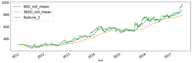
Just like groupby and resample, you can calculate multiple metrics with the agg function for each window.
6.2 Expanding window functions
Another type of window function deals with expanding windows. Each new window will contain all the records up to the current date:
Expanding windows are useful for calculating ‘running’ metrics-for example, running sum, mean, min and max, running rate of return, etc.
Below, you will see how to calculate the cumulative sum. The cumulative sum is actually an expanding window function with a window size of 1:
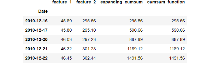
expanding function has a min_periods parameter that determines the initial window size.
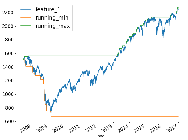
Now, let’s see how to plot the running min and max:
Summary
I think congratulations are in order!
Now, you know every single Pandas function you can use to manipulate time-series data. It has been an excruciatingly long post, but it was definitely worth it since now, you can tackle any time series data thrown at you.
This post was mainly focused on data manipulation. The next posts in the series will be about more in-depth time series analyses, similar posts on every single plot you can create on time series, and dedicated articles on forecasting. Stay tuned!
Loved this article and, let’s face it, its bizarre writing style? Imagine having access to dozens more just like it, all written by a brilliant, charming, witty author (that’s me, by the way :).
For only 4.99$ membership, you will get access to not just my stories, but a treasure trove of knowledge from the best and brightest minds on Medium. And if you use my referral link, you will earn my supernova of gratitude and a virtual high-five for supporting my work.


