Essential Statistics to Evaluate the Performance of Financial Advice

Robert C. Merton, Professor of Finance at MIT and 1997 Nobel Laureate in Economics commented in a talk (https://www.youtube.com/watch?v=uYABw7h07tc Minute 12:50) that financial advice is not verifiable given a portfolio manager’s track record because it takes somewhere between 40 and 400 years to get a t-statistic of 2 — the minimum for significance! I was surprised when I heard this and wondered how this was computed. In addition, if we can’t tell if an investor is good or bad based on his/her past performance, can we tell if an investing or trading strategy is good or bad, statistically? The purpose of this article is to answer these critical questions that every investor or trader is intrigued to know.

Let me give a real-world finance problem so that you get an exact idea of what we are trying to do here. You, as a day trader, developed a new trading strategy that gave you a daily percent return of 0.82, 0.94, 0.96, 1.31, 0.94, 1.21, 1.26, 1.09, 1.13, and 1.14 over the past 10 trading days while your current trading strategy gave you a list of daily percent returns as 0.94, 1.09, 0.97, 0.98, 1.14, 0.85, 1.30, 0.89, 0.87, and 1.01. The question is: should you abandon your current strategy and adopt your new strategy? This is a piece of financial advice you want to receive from an advisor who might be an expert, yourself, your AI, or someone else.

As usual, we need to have some theoretical preparations before we delve into the problem-solving part using code.

1. Theoretical Foundation

Someone might say: okay, this is a simple problem. We can compare the means of the two strategies. The means of percent returns are 1.08 and 1.004 for the new and current strategies, respectively. Since 1.08 > 1.004, the new strategy is better, and the current strategy can be abandoned.

Such a solution is problematic in many aspects. Since we only have 10 days of data, how do we know the mean we computed is the mean of percent returns of the future that may have 250 trading days per year x 40 years (assume we trade 40 years and then retire, can we?) = 10,000 trading days or more? If we can’t be certain about the mean, how can we draw a conclusion based on the mean, let alone the variances?

After we realize the problem is not simple, let’s start with the essential statistics for investors and traders.

1.1 Central Limit Theorem and Normal Distribution

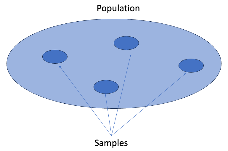
When producing a point estimate of a population statistic, for this case, the mean of percent returns for a strategy over the entire trading career, the value of a point estimate (i.e., the mean in this example) depends on which sample, out of all the possible samples, happens to be selected (Fig. 1). Different samples usually yield different estimates as a result of chance differences from one sample to another. Because of sampling variability, rarely is the point estimate (i.e., the mean of percent returns) from a sample exactly equal to the true value of the population characteristic. However, we can still make an inference about the mean of percent returns for a strategy over the entire trading career with the following statistics theories.

Let x_bar be the mean of the sample and n be the sample size. Statisticians have proved that if n is large (generally greater than or equal to 30), regardless of the population distribution, x_bar simply follows a normal distribution. This is called “Central Limit Theorem”.

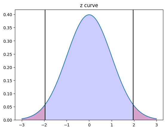
This theorem makes our inference much easier because the bell-shaped normal distribution curve (Fig. 2) is pretty standard. From the normal curve (z curve), we know the (blue) area under the curve within 2 (or 1.96 to be precise) standard deviations of the mean is 95%. A lot of statistical decisions can be made based on these numbers. If an instance falls into the blue area, we say the instance is not significant because, for 95% of the chance, we get a similar instance. However, if an instance falls into the two-tailed regions (the red areas), we say the instance is significant because it rarely occurs with a remaining 5% of chance. Therefore, in statistics, we usually set a significance level of 0.05. We will do this too in this article to distinguish the performance of one piece of financial advice from another.

1.2 Statistic

The threshold (critical) values of ±1.96 on the x-axis for separating the z-curve are examples of z-statistic. To tell if an instance is significant, we need to compute the z-statistic using Formula 1. If the z-stat is less than -1.96 or greater than 1.96, the instance falls into the two-tailed regions, indicating significance. A p-value that denotes the probability under the assumption of insignificance will be less than the significance level (alpha) of 0.05.

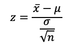
where x_bar is the mean of the sample, mu is the mean of the population, sigma is the standard deviation of the population, and n is the sample size.

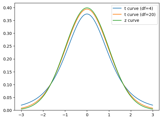
Since the z-curve is obtained when the sample size is greater than or equal to 30, what about our case where our sample size is just 10? Well, the z-curve cannot be used. We will need to use the t-curve. T-curves are properties of t distributions. Different sample sizes will give us different bell-shaped t-curves. A concept of degrees of freedom (abbreviated as df), which is linearly correlated with sample sizes, is used to control the shape of the t-curves. As shown in Fig. 3, which compares the z curve with the t curves for 4 df and 20 df, the larger the number of df (or sample size), the more closely the t curve resembles the z curve. Since the df-dependent t-curves have different shapes, the threshold (critical) values to determine the significance level of 0.05 are no longer ±1.96 but are greater than these numbers (Fig. 4) and need to be read from the t-tables. In addition, instead of z-statistic, we need to compute t-statistic using Formula 2 so that the computed t-stat can be compared with the threshold (critical) values to determine the significance.

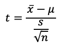
where x_bar is the mean of the sample, mu is the mean of the population, s is the standard deviation of the sample, and n is the sample size.

1.3 The Required Sample Size

Since the sample size matters, what would be the required sample size if we want to estimate a population mean to be within bound B with 95% confidence? This answers how Prof. Robert Merton reached his conclusion that 40–400 years of records are needed to prove a good portfolio manager. We can use Formula 3 to determine the required sample size.

where n is the required sample size, sigma is the standard deviation of the population, and B is the bound on the error of estimation.

Note that in practice the standard deviation of the population is unknown, and we only know the standard deviation of the sample. We could (1) either use the standard deviation of the sample to replace sigma for estimation (2) or use (range of the sample)/4 to estimate sigma.

1.4 Hypothesis Testing

A test of hypothesis is a method that uses sample data to decide between two competing claims (hypotheses) about a population characteristic. The null hypothesis, denoted by H0, is a claim about a population characteristic that is initially assumed to be true. The alternative hypothesis, denoted by Ha, is the competing claim. In carrying out a test of H0 versus Ha, the hypothesis H0 will be rejected in favor of Ha if the p-value is less than the significance level of 0.05.

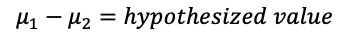
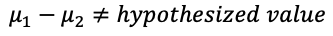
For our context, the null hypothesis H0 could be: Strategy 1’s mean of percent returns = Strategy 2’s mean of percent returns, or mu1 = mu2, or mu1 — mu2 = 0. And the alternative hypothesis Ha is: mu1 != mu2 or mu1-mu2 != 0.

The subsequent steps are to compute the t-statistic (if the population’s standard deviation sigma is unknown) or z-statistic (if the population’s standard deviation sigma is known), and then compute the p-value as an area under the t-curve or z-curve. For a p-value of less than the significance level we set, we can reject the null hypothesis H0 and embrace the alternate hypothesis Ha.

1.5 Two-tailed test vs. one-tailed test

What happens if we desire an alternative hypothesis of mu1 > mu2, not mu1 != mu2, like the example in this article? A common misbelief is to use a one-tailed test instead of a two-tailed test. The consequence is that you miss an effect in the other direction, which is mu1 < mu2. We must understand when a one-tailed test is appropriate.

In our context, you have developed a new trading strategy that you believe is an improvement over your existing trading strategy. You wish to maximize your ability to detect the improvement, so you are thinking of opting for a one-tailed test. In doing so, you fail to test for the possibility that the new strategy is worse than the existing strategy. The consequence of this extreme is dangerous. Therefore, this is an inappropriate use of a one-tailed test.

Imagine again that you have developed a new drug. It is cheaper than the existing drug and, you believe, no less effective. In testing this drug, you are only interested in testing if it is less effective than the existing drug. You do not care if it is significantly more effective. In other words, there is no consequence for the other extreme. In this scenario, a one-tailed test would be appropriate.

To learn more about the differences between two-tailed and one-tailed tests, you may visit this link. But in the context of our example in this article, we will use a two-tailed test to be safe.

1.6 Steps of the Two-Sample t-Test for Comparing Two Population Means

The following is a summary of such a two-sample t-test that we will perform on our data. It requires the two samples to be independently selected.

• Step 1: Define hypotheses.

Null hypothesis H0:

Alternative hypothesis Ha:

• Step 2: Calculate the test statistic.

• Step 3: Calculate the degrees of freedom.

where

• Step 4: Calculate the p-value as an area under the t-curve. For a p-value of less than the significance level we set, we can reject the null hypothesis H0 and embrace the alternate hypothesis Ha.

In our case, the hypothesized value can be set to zero. Note that all mus denote the means of the populations, all x_bars denote the means of the samples, and all s values denote the standard deviations of the samples.

Now, let’s code a system to handle the statistical computations.

2. Code Implementation

2.1 The Demo Problem

First, we import the NumPy, Matplotlib, SciPy, and yfinance libraries. We mainly use SciPy’s stats sub-package to handle the statistical computations.

import numpy as np
import matplotlib.pyplot as plt
from scipy import stats
from scipy.stats import t,norm
import yfinance as yf

Then we create two data groups. Data Group 1 stores Strategy 1 (the new strategy)’s percent returns and Data Group 2 stores Strategy 2 (the current strategy)’s percent returns.

# Creating data groups
data_group1 = np.array([0.82,0.94,0.96,1.31,0.94,1.21,1.26,1.09,1.13,1.14])
data_group2 = np.array([0.94,1.09,0.97,0.98,1.14,0.85,1.30,0.89,0.87,1.01])
 
# Print the numbers of both data groups
print(len(data_group1), len(data_group2)) # output is 10 10

# Print the mean of both data groups
print(np.mean(data_group1), np.mean(data_group2)) # output is 1.08 1.004

# Print the standard deviation of both data groups
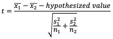
print(np.std(data_group1), np.std(data_group2)) # output is 0.1515255753990065 0.13192422067232387

In case you are curious about what the actual equity curves look like with the two strategies, you can translate the two lists of percent returns into the equity curves with the following code.

start_fund = 100
strategy1 = start_fund*np.ones(len(data_group1)+1)
strategy2 = start_fund*np.ones(len(data_group2)+1)

for i in range(1,len(data_group1)+1):
    strategy1[i]=strategy1[i-1]*(1+data_group1[i-1]/100)

for i in range(1,len(data_group2)+1):
    strategy2[i]=strategy2[i-1]*(1+data_group2[i-1]/100)

plt.plot(range(len(strategy1)),strategy1,label='Strategy 1')
plt.plot(range(len(strategy2)),strategy2,label='Strategy 2')
plt.legend()
plt.xlabel('Days')
plt.ylabel('Equity')
plt.show()

It turns out that within 10 trading days, Strategy 1 resulted in a higher equity value than Strategy 2. So, intuitively, people tend to conclude that Strategy 1 is better than Strategy 2. But we let the statistics take care of the performance evaluation.

Option 1: we can employ SciPy’s pre-programmed “stats.ttest_ind” function to take care of the two-sample t-test computations. It is as simple as a one-liner.

# Perform the two sample t-test
tstat, pvalue = stats.ttest_ind(a=data_group1, b=data_group2, equal_var=False)
print(tstat, pvalue) # output is 1.1348481349355801 0.27160348695265546

With a t-stat of 1.13 and the resultant p-value of 0.27, which is greater than the significance level of 0.05, we cannot reject the null hypothesis. So, there is no sufficient evidence to say Strategy 1 is better!

Option 2: we can code the algorithm as outlined in Section 1.6. We get the same result.

# Two-sample t test for comparing two population means
mu1,mu2,B = np.mean(data_group1),np.mean(data_group2),0 # B is hypothesized value
s1,s2 = np.std(data_group1),np.std(data_group2)
# s1,s2 = (np.max(data_group1)-np.min(data_group1))/4,(np.max(data_group2)-np.min(data_group2))/4
n1,n2 = len(data_group1),len(data_group2)
v1,v2 = s1**2/n1,s2**2/n2
tstat = (mu1-mu2-B)/np.sqrt(v1+v2)
df = (v1+v2)**2/(v1**2/(n1-1)+v2**2/(n2-1))
if tstat < 0:
    pvalue = 2*t.cdf(tstat, df = df)
else:
    pvalue = 2*t.sf(tstat, df = df)
print(tstat,df,pvalue) # output is 1.1962349682635118 17.66529895322754 0.2474145239902979

2.2 Merton’s Problem

Now, let’s compute the years required to tell if a portfolio manager is good. Prof. Merton said it requires 40–400 years.

Let’s say I am a portfolio manager who simply buys and holds the large-cap stock index fund “SPY”. And I tell a potential client that if he/she gives his/her money to me to manage, I will guarantee to make money for him/her. I add that I have 22 years of track record, assuming that I held “SPY” since the year 2000 when I could buy “SPY” at $148 per share, and by the end of 2022 it is worth $382 per share. In other words, the portfolio I managed resulted in a 158% return over 22 years. So, please trust me.

You, as the potential client, need to evaluate this financial advice of giving your money to me to manage. Let’s say your bottom line is I do not lose money!

First, you look at my history closely. You download the “SPY” from 2000 to 2022 as the track record of the portfolio I managed.

df = yf.download('SPY',start='2000-01-01',end='2022-12-31',interval='1mo')
df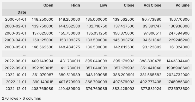

Since yfinance only gave monthly data, you need to aggregate the monthly data into the annual data.

dfy = df.resample('1y').agg({'Open': 'first', 'High': 'max', 'Low': 'min', 'Close': 'last','Volume':'sum'})
dfy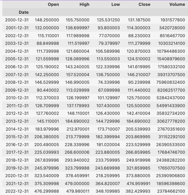

You can also visualize the data. At first glance, this looks amazing!

plt.plot(dfy.index,dfy.Close)
plt.ylabel('Price in USD')
plt.title('SPY')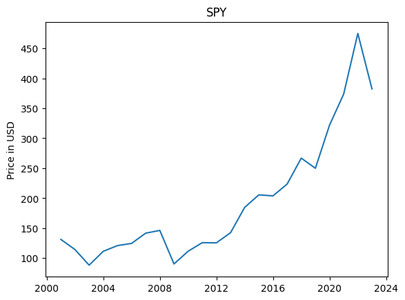

But wait a minute, let’s dismantle the data into the annual percent returns like the demo problem shows and call it the benchmark.

benchmark = np.zeros(len(dfy))
benchmark[0] = (dfy.Close.iloc[0]-dfy.Open.iloc[0])/dfy.Open.iloc[0]*100
for i in range(1,len(benchmark)):
    benchmark[i] = (dfy.Close.iloc[i]-dfy.Close.iloc[i-1])/dfy.Close.iloc[i-1]*100
print(np.mean(benchmark),np.std(benchmark)) # output is 5.835749474294194 17.54861542481561

plt.plot(dfy.index,benchmark)
plt.ylabel('Annual Percent Return')
plt.show()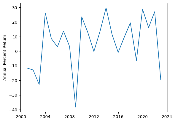

Well, you can see the mean of the sample’s annual percent returns is 5.83 and the standard deviation is 17.54. Since your bottom line is I don’t lose money, to translate this language to a statistics problem, you want to ensure the mean of 5.83 plus minus the bound of error must be greater than 0. In other words, the bound of error B = 5.83, which is the mean of the sample’s annual percent returns.

Now, you can employ Formula 3 to compute the required sample size.

(1.96*np.std(benchmark)/np.mean(benchmark))**2 # output is 34.73798127302209

est_std = (np.max(benchmark)-np.min(benchmark))/4
(1.96*est_std/np.mean(benchmark))**2 # output is 32.57068044057159

Using different methods to estimate the standard deviation of the population, we get either 35 or 33, meaning I need a record of 35 years to confidently say I will not lose money for you. A record of 22 years is not enough for you to trust me!

What about I want to make an ambitious claim that I am confident to make a 4% annual return for you as a minimum using a strategy of buy-and-hold “SPY”? In this case, the bound of error is computed as 5.83–4 = 1.83. Using Formula 3, we get 353, meaning I need a record of 353 years to confidently say that!

(1.96*np.std(benchmark)/1.83)**2 # output is 353.2609857043022

2.3 Code for Generating Fig. 2–4

In case you are interested, the followings are the code for generating Fig. 2–4.

Code for Fig. 2.

x = np.linspace(-3,3,100)
plt.plot(x, norm.pdf(x),label='z curve')
plt.axvline(norm.ppf(0.025),c='k')
plt.axvline(norm.ppf(0.975),c='k')
plt.fill_between(x, 0, stats.norm.pdf(x,), color='blue', alpha=.2)
plt.fill_between(x[x<norm.ppf(0.025)],0,norm.pdf(x[x<norm.ppf(0.025)]), color='red', alpha=.2)
plt.fill_between(x[x>norm.ppf(0.975)],0,norm.pdf(x[x>norm.ppf(0.975)]), color='red', alpha=.2)
plt.ylim([0, None])
plt.title('z curve')
plt.show()

Code for Fig. 3.

df = 4
plt.plot(x, t.pdf(x, df),label='t curve (df=4)')

df = 20
plt.plot(x, t.pdf(x, df),label='t curve (df=20)')

plt.plot(x,norm.pdf(x),label='z curve')
plt.ylim([0,None])
plt.legend()
plt.show()

Code for Fig. 4.

df = 20
plt.plot(x, t.pdf(x, df),label='t curve (df=20)')
plt.axvline(t.ppf(0.025,df),c='k')
plt.axvline(t.ppf(0.975,df),c='k')
plt.fill_between(x, 0, t.pdf(x, df), color='blue', alpha=.2)
plt.fill_between(x[x<t.ppf(0.025,df)],0,t.pdf(x[x<t.ppf(0.025,df)], df), color='red', alpha=.2)
plt.fill_between(x[x>t.ppf(0.975,df)],0,t.pdf(x[x>t.ppf(0.975,df)], df), color='red', alpha=.2)
plt.ylim([0, None])
plt.title('t curve (df=20)')
plt.show()

Concluding Remarks

Essential statistics knowledge is needed for every investor and trader to make informed financial decisions. What you see in the equity curves and track records may cheat you, but statistical science will not. In Prof. Merton’s talk, he added that since financial advice is not verifiable, what the clients need from a portfolio manager is simply trust. At the end of this article, I would also like to add that it is much easier to evaluate the performance of a trading strategy if done correctly because the back-test and forward-test easily allow us to have greater than or equal to 30 data, which are the industry standard to satisfy the normal distribution approximations. This is especially true for day traders.

Disclaimer:

I do not make any guarantee or other promise as to any results that are contained within this article. You should never make any investment decision without first consulting with your financial advisor and conducting your own research and due diligence. To the maximum extent permitted by law, I disclaim any implied warranties of merchantability and liability in the event any information contained in this article proves to be inaccurate, incomplete, or unreliable or results in any investment or other losses.

I hope you enjoy reading the article. I periodically publish articles of original content on the applications of machine learning and deep learning in the realms of quantitative trading, finance, and engineering. I’m also writing my book Day Trade with AI, which is to be released soon. If you finish reading here and would like to see more of my writings, you may subscribe for free to get notified when I publish a new story. And let’s connect!

📚 Medium | 🐦 Twitter | 👥 Linkedin

To support me, you can buy me a coffee. I drink a lot of coffee while writing!

Want to read more than 3 free stories a month? — Become a Medium member for $5/month. You may use my referral link when you sign up. I’ll receive a commission at no extra cost to you.