
Ensemble Oversampling And Under-Sampling For Imbalanced Classification Using Python
Combining ensemble tree models with over and under-sampling techniques to improve imbalanced classification results

Ensemble oversampling and under-sampling combine ensemble tree models with over and under-sampling techniques to improve imbalanced classification results.
This tutorial uses the Python library imblearn to compare different ensemble oversampling and under-sampling models, and choose the best model for the imbalanced dataset. You will learn
- How to use a balanced random forest classifier?
- How to use a random under-sampling boosting classifier?
- How to use an easy ensemble classifier with a boost?
- How to use a balanced bagging classifier with Near Miss under-sampling?
- How to use a balanced bagging classifier with SMOTE?
- How to pick the best model based on performance metrics?
Resources for this post:
- Video tutorial on YouTube
- Python code is at the end of the post. Click here for the notebook.
- More video tutorials on imbalanced modeling and anomaly detection
- More posts on anomaly detection and imbalanced classification
Let’s get started!
Step 1: Install And Import Libraries
We will use a Python library called imbalanced-learn to handle imbalanced datasets, so let’s install the library first.
# Install the imbalanced learn library
pip install -U imbalanced-learn
The following text shows the successful installation of the imblearn library. Based on when you run the installation, your version of the package may be different from mine.
Successfully installed imbalanced-learn-0.8.0 scikit-learn-0.24.2 threadpoolctl-2.2.0Now let’s import the Python libraries.
# Synthetic dataset
from sklearn.datasets import make_classification
# Data processing
import pandas as pd
import numpy as np# Data visualization
import matplotlib.pyplot as plt
import seaborn as sns
from collections import Counter# Model and performance
from sklearn.model_selection import train_test_split, cross_validate
from sklearn.ensemble import RandomForestClassifier
from sklearn.metrics import classification_report# Ensembled sampling
from imblearn.under_sampling import NearMiss
from imblearn.over_sampling import SMOTE
from imblearn.ensemble import BalancedRandomForestClassifier
from imblearn.ensemble import RUSBoostClassifier
from imblearn.ensemble import EasyEnsembleClassifier
from imblearn.ensemble import BalancedBaggingClassifierStep 2: Create an Imbalanced Dataset
Using `make_classification` from the sklearn library, We created two classes with the ratio between the majority class and the minority class being 0.995:0.005. Two informative features were made as predictors. We did not include any redundant or repeated features in this dataset.
# Create an imbalanced dataset
X, y = make_classification(n_samples=100000, n_features=2, n_informative=2,
                           n_redundant=0, n_repeated=0, n_classes=2,
                           n_clusters_per_class=1,
                           weights=[0.995, 0.005],
                           class_sep=0.5, random_state=0)
# Convert the data from numpy array to a pandas dataframe
df = pd.DataFrame({'feature1': X[:, 0], 'feature2': X[:, 1], 'target': y})# Check the target distribution
df['target'].value_counts(normalize = True)The output shows that we have about 1% of the data in the minority class and 99% of the data in the majority class.
0    0.9897
1    0.0103
Name: target, dtype: float64
Let’s visualize the imbalanced data we just created using a scatter plot.
# Visualize the data
plt.figure(figsize=(12, 8))
sns.scatterplot(x = 'feature1', y = 'feature2', hue = 'target', data = df)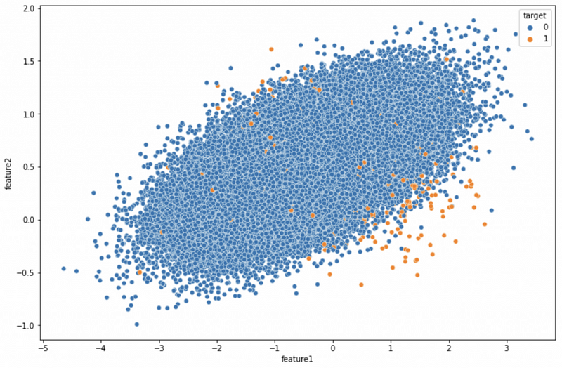
Step 3: Train Test Split
In this step, we split the dataset into 80% training data and 20% validation data. random_state ensures that we have the same train test split every time. The seed number for random_state does not have to be 42, and it can be any number.
# Train test split
X_train, X_test, y_train, y_test = train_test_split(X, y, test_size=0.2, random_state=42)
# Check the number of records
print('The number of records in the training dataset is', X_train.shape[0])
print('The number of records in the test dataset is', X_test.shape[0])
print(f"The training dataset has {sorted(Counter(y_train).items())[0][1]} records for the majority class and {sorted(Counter(y_train).items())[1][1]} records for the minority class.")The train test split gives us 80,000 records for the training dataset and 20,000 for the validation dataset. Thus, we have 79,183 data points from the majority class and 817 from the minority class in the training dataset.
The number of records in the training dataset is 80000
The number of records in the test dataset is 20000
The training dataset has 79183 records for the majority class and 817 records for the minority class.
Step 4: Baseline Model Without Sampling
We use cross-validation to evaluate the model performance and use minority class recall as the north star metric.
# Train the random forest model using the imbalanced dataset
rf = RandomForestClassifier()
baseline_model_cv = cross_validate(rf, X_train, y_train, cv = 5, n_jobs = -1, scoring="recall")
# Check the model performance
print(f"{baseline_model_cv['test_score'].mean():.3f} +/- {baseline_model_cv['test_score'].std():.3f}")The 5-fold cross-validation gives the recall value of 0.04 and the standard deviation of 0.018. This shows that the model only captured 4% of the minority class.
Step 5: Balanced Random Forest Classifier
The Python imbalanced learn library has BalancedRandomForestClassifier that can automatically under-sample the dataset when bootstrapping from the training dataset to build each decision tree.
random_state makes the random sampling reproducible.
Using cross_validate with cv = 5 implements 5-fold cross-validation. n_jobs = -1 is for parallel processing. scoring="recall" tells the cross-validation that the score we are interested in is 'recall'.
# Train the balanced random forest model
brf = BalancedRandomForestClassifier(random_state=42)
brf_model_cv = cross_validate(brf, X_train, y_train, cv = 5, n_jobs = -1, scoring="recall")
# Check the model performance
print(f"{brf_model_cv['test_score'].mean():.3f} +/- {brf_model_cv['test_score'].std():.3f}")0.557 +/- 0.043The BalancedRandomForestClassifier gives us the recall value of 0.557, which is a big improvement from the baseline model.
Step 6: Random Under-Sampling Boosting Classifier
RUSBoostClassifier uses random under-sampling for the boosted trees.
# Train the random under-sampling boosting classifier model
rusb = RUSBoostClassifier(random_state=42)
rusb_model_cv = cross_validate(rusb, X_train, y_train, cv = 5, n_jobs = -1, scoring="recall")
# Check the model performance
print(f"{rusb_model_cv['test_score'].mean():.3f} +/- {rusb_model_cv['test_score'].std():.3f}")The RUSBoostClassifier gives us the recall value of 0.456, which is much better than the baseline model, but not as good as the balanced random forest classifier.
0.456 +/- 0.067Step 7: Easy Ensemble Classifier for Ada Boost Classifier
The Python imbalanced learn library has a specific method called EasyEnsembleClassifier for the AdsBoostClassifier.
# Train the easy ensemble classifier model
eec = EasyEnsembleClassifier(random_state=42)
eec_model_cv = cross_validate(eec, X_train, y_train, cv = 5, n_jobs = -1, scoring="recall")
# Check the model performance
print(f"{eec_model_cv['test_score'].mean():.3f} +/- {eec_model_cv['test_score'].std():.3f}")The EasyEnsembleClassifier gives us the average recall values of 0.542, which is slightly lower than the balanced random forest calssifier. However, the standard deviation of 0.029 is smaller than the balanced random forest calssifier standard deviation.
0.542 +/- 0.029Step 8: Balanced Bagging Classifier — Near Miss Under Sampling
BalancedBaggingClassifier gives us more flexibility to use different base models and samplers. The default base model is the decision tree model. We use Near Miss under-sampling as the sampler in this step.
Near Miss has three versions. We use version 3, which first keeps M nearest neighbors of the minority data, then select the majority data for which the average distance to the N nearest neighbors is the largest.
# Train the balanced bagging classifier model using near miss under sampling
bbc_nm = BalancedBaggingClassifier(random_state=42, sampler=(NearMiss(version=3)))
bbc_nm_model_cv = cross_validate(bbc_nm, X_train, y_train, cv = 5, n_jobs = -1, scoring="recall")
# Check the model performance
print(f"{bbc_nm_model_cv['test_score'].mean():.3f} +/- {bbc_nm_model_cv['test_score'].std():.3f}")The 5-fold cross-validation gives us the average recall value of 0.504, which is much better than the baseline model but not as good as the balanced random forest classifier.
0.504 +/- 0.019Step 9: Balanced Bagging Classifier — SMOTE
In this step, we changed the sampler from NearMiss under-sampling to SMOTE oversampling.
# Train the balanced bagging classifier model using SMOTE
bbc_smote = BalancedBaggingClassifier(random_state=42, sampler=(SMOTE()))
bbc_smote_model_cv = cross_validate(bbc_smote, X_train, y_train, cv = 5, n_jobs = -1, scoring="recall")
# Check the model performance
print(f"{bbc_smote_model_cv['test_score'].mean():.3f} +/- {bbc_smote_model_cv['test_score'].std():.3f}")The BalancedBaggingClassifier using SMOTE oversampling gives us the recall of 0.109, which is better than the baseline model but much worse than the models using the under-sampling techniques.
0.109 +/- 0.034Step 10: Use Best Model On Training Dataset
From the comparison above, we can see that the ensemble models using under-sampling generally perform better than oversampling.
The Balanced Random Forest Classifier has the highest recall value among the ensemble methods we compared, so we will use it to train the final model.
Notice that we are using the whole training dataset to train the model and use the testing dataset to make predictions.
# Train the balanced random forest model
brf = BalancedRandomForestClassifier(random_state=42)
brf_model = brf.fit(X_train, y_train)
brf_prediction = brf_model.predict(X_test)
# Check the model performance
print(classification_report(y_test, brf_prediction))The model captures 51% of the minority class in the testing dataset.
precision recall f1-score support 0 0.99 0.62 0.76 19787
1 0.01 0.51 0.03 213 accuracy 0.62 20000
macro avg 0.50 0.56 0.39 20000
weighted avg 0.98 0.62 0.75 20000In comparison, the baseline random forest model on the imbalanced dataset has 3% recall for the minority class, so the ensemble method gave us a 48% increase in recall.
# Train the baseline random forest model
rf = RandomForestClassifier()
baseline_model = rf.fit(X_train, y_train)
baseline_prediction = baseline_model.predict(X_test)
# Check the model performance
print(classification_report(y_test, baseline_prediction))precision recall f1-score support 0 0.99 1.00 0.99 19787
1 0.50 0.03 0.06 213 accuracy 0.99 20000
macro avg 0.74 0.52 0.53 20000
weighted avg 0.98 0.99 0.98 20000Summary
In this tutorial, we compared different ensemble oversampling and undersampling models for imbalanced datasets. You learned
- How to use a balanced random forest classifier?
- How to use a random under-sampling boosting classifier?
- How to use an easy ensemble classifier with ada boost?
- How to use a balanced bagging classifier with Near Miss under-sampling?
- How to use a balanced bagging classifier with SMOTE?
- How to pick the best model based on performance metrics?
More tutorials are available on GrabNGoInfo YouTube Channel and GrabNGoInfo.com.
Recommended Tutorials
- GrabNGoInfo Machine Learning Tutorials Inventory
- One-Class SVM For Anomaly Detection
- 3 Ways for Multiple Time Series Forecasting Using Prophet in Python
- Four Oversampling And Under-Sampling Methods For Imbalanced Classification Using Python
- Multivariate Time Series Forecasting with Seasonality and Holiday Effect Using Prophet in Python
- How to detect outliers | Data Science Interview Questions and Answers
- Time Series Anomaly Detection Using Prophet in Python


