Energy consumption time series forecasting with python and LSTM deep learning model

How to use deep learning with time series

The objective of this article is to present the reader with a class in python that has a very intuitive and easy input to model and predict time series data using deep learning. Ideally, the reader should be able to copy the code presented in this article or the GitHub repository, tailor it to his needs (add more layers to the model for example) and use it his/her work.

All the code that is used in this article can be found here:

https://github.com/Eligijus112/deep-learning-ts

The data for this article can be found here:

https://www.kaggle.com/robikscube/hourly-energy-consumption

The packages that are used for deep modeling are TensorFlow and Keras.

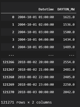
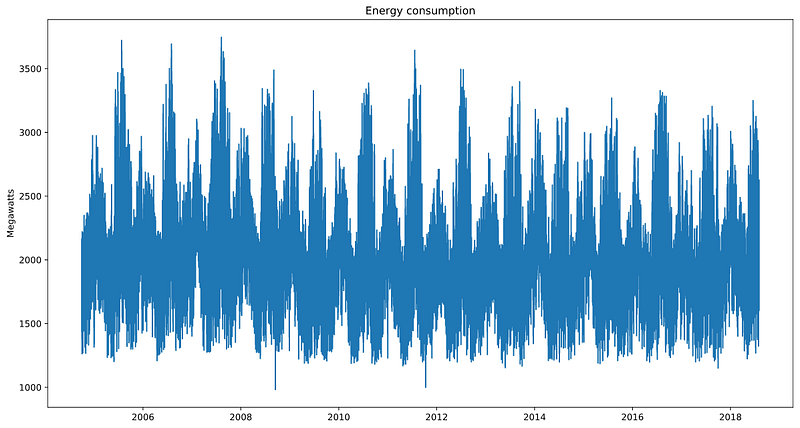
A time series is a sequence of numerical data points in successive order. These points are often measured at regular intervals (every month, every day, every hour, etc.). The data frequency used in this article is hourly and it was measured from 2004–10–01 to 2018–08–03. The total number of raw data points is 121271.

Visualization of the time series:

The main objective of the deep learning algorithm for a given time series is to find a function f such that:

Yₜ = f(Yₜ₋₁, Yₜ₋₂, …, Yₜ₋ₚ)

In other words, we want to estimate a function that explains the current values of energy consumption based on p lags of the same energy consumption.

This article is not about explaining why long short-term memory (LSTM) deep learning networks are good for time series modeling or how it works. For resources on that check great articles like:

For the implementation of LSTM (or any RNN layer) in Keras see the official documentation:

Firstly, we need to read the data :

We then need a function that converts the time series into an X and Y matrices for the deep learning model to start learning. Let us say that we want to create a function that explains current time series values using 3 lags:

Yₜ = f(Yₜ₋₁, Yₜ₋₂, Yₜ₋₃)

And we have this data:

ts = [1621.0, 1536.0, 1500.0, 1434.0, 1489.0, 1620.0]

What we would like is to create two matrices:

X = [
[1621.0, 1536.0, 1500.0], # First three lags
[1536.0, 1500.0, 1434.0], # Second three lags
[1500.0, 1434.0, 1489.0], # Third three lags
]

Y = [1434.0, 1489.0, 1620.0]

This is the most important trick when using deep learning with time series. You can feed these X and Y matrices not only to a recurrent neural network system (like LSTM) but to any vanilla deep learning algorithm.

The deep learning model has an LSTM layer (that serves as the input layer as well) and an output layer.

During my searches on the internet for an easy to use deep learning model with time series I came across various articles that picked apart several parts of modeling like how to define a model, how to create the matrix for the models, etc. I did not find a package or a class that wrapped everything up into one easy to use entity. So I decided to do that myself:

Initiating the class:

# Initiating the class

deep_learner = DeepModelTS(
data = d,
Y_var = 'DAYTON_MW',
lag = 6,
LSTM_layer_depth = 50,
epochs = 10,
batch_size = 256,
train_test_split = 0.15
)

The parameters for the class are:

data - the data used for modeling.

Y_var - the variable name we want to model/forecast.

lag - the number of lags used for modeling.

LSTM_layer_depth - number of neurons in the LSTM layer.

epochs - number of training loops (forward propagation to backward propagation cycles).

batch_size - the size of the data sample for the gradient descent used in the finding of the parameters by the deep learning model. All the data is divided into chunks of batch_size sizes and fed through the network. The internal parameters of the model are updated after each batch_size of data goes forward and backward in the model.

To read more about epochs and batch sizes visit:

train_test_split - the share of the data that is used for testing. 1 - train_test_split is used for the training of the model.

Fitting the model:

# Fitting the model

model = deep_learner.LSTModel()

After the above command, you can witness the fan-favorite training screen:

Training the model with more lags (hence, a larger X matrix) increases the training time:

deep_learner = DeepModelTS(
data = d,
Y_var = 'DAYTON_MW',
lag = 24, # 24 past hours are used
LSTM_layer_depth = 50,
epochs = 10,
batch_size = 256,
train_test_split = 0.15
)

model = deep_learner.LSTModel()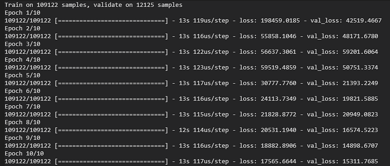

Now that we have a created model we can start forecasting. The formula for the forecasts with a model trained with p lags:

Yₜ₊₁ = f(Yₜ, Yₜ₋₁, …, Yₜ₋ₚ₊₁)

# Defining the lag that we used for training of the model 
lag_model = 24

# Getting the last period
ts = d['DAYTON_MW'].tail(lag_model).values.tolist()

# Creating the X matrix for the model
X, _ = deep_learner.create_X_Y(ts, lag=lag_model)

# Getting the forecast
yhat = model.predict(X)

If the data was split into training and test sets then the deep_learner.predict() method will predict the points which are in the test set to see how our model performs out of sample.

yhat = deep_learner.predict()

# Constructing the forecast dataframe
fc = d.tail(len(yhat)).copy()
fc.reset_index(inplace=True)
fc['forecast'] = yhat

# Ploting the forecasts
plt.figure(figsize=(12, 8))
for dtype in ['DAYTON_MW', 'forecast']:

  plt.plot(
    'Datetime',
    dtype,
    data=fc,
    label=dtype,
    alpha=0.8
  )

plt.legend()
plt.grid()
plt.show()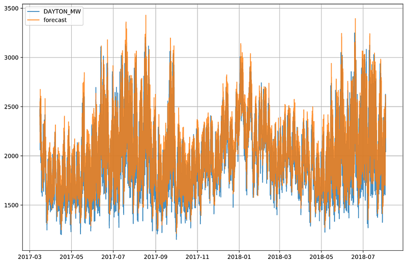

As we can see, the forecasts for 15 percent of the data that was hidden from model creation are close to the real values.

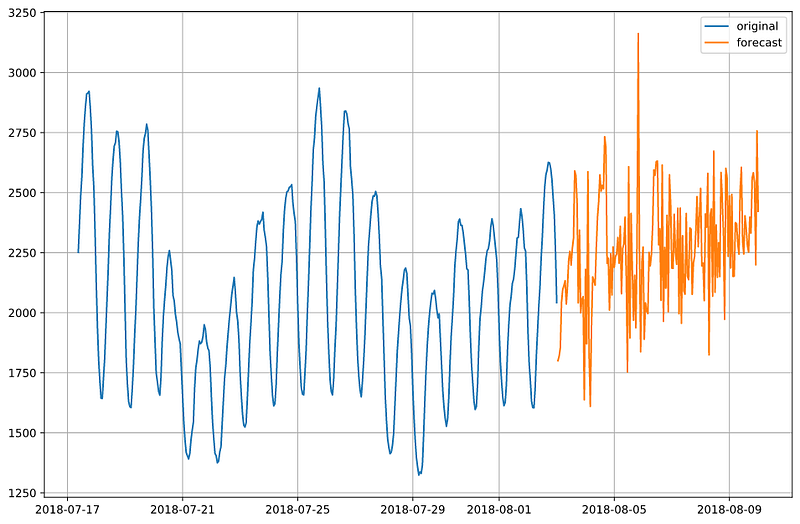
We usually want to forecast ahead of the last original time series data. The class DeepModelTS has the method predict_n_ahead(n_ahead) which forecasts n_ahead time steps.

# Creating the model using full data and forecasting n steps aheaddeep_learner = DeepModelTS(
data=d,
Y_var='DAYTON_MW',
lag=48,
LSTM_layer_depth=64,
epochs=10,
train_test_split=0
)

# Fitting the model
deep_learner.LSTModel()

# Forecasting n steps ahead
n_ahead = 168

yhat = deep_learner.predict_n_ahead(n_ahead)
yhat = [y[0][0] for y in yhat]

The above code forecasts one week's worth of steps ahead (168 hours). Comparing it with the previous 400 hours:

In conclusion, this article presented a simple pipeline example when working with modeling and forecasting of the time series data:

Reading and cleaning the data (1 row for 1 time step)

Selecting the number of lags and model depth

Initiating the DeepModelTS() class

Fitting the model

Forecasting n_steps ahead

I hope that the reader can use the code showcased in this article in his/her professional and academic work.