
The Laws of Large Numbers
Weak vs. strong: unpacking the secret of convergence of random variables
In this post, two versions of the laws of large numbers (later LLN for short) are discussed. Both say that in repeating independent experiments, the sample mean tends to be close to the population mean, but there are subtle differences between them. We will explore those differences with examples. Also, those LLNs are closely connected with the convergence of sequences of random variables (later r. v. for short).
Regarding the common confusion about “distribution,” in this post, when “distribution” is used, it means the probability mass/density function (PMF/PDF) and “cumulative distribution function” (CDF) is used instead of “distribution function.” (I completely agree that the term “distribution function” is confusing.)
Some preparation
Here is some knowledge that will be referred to later. You can skip this section and go to the LLN directly. It’s just that, from experience, backward references are much more pleasant than forward references.
Inequalities
Firstly, there are two famous inequalities in probability theory worth mentioning, at least briefly — the Markov inequality and Chebyshev’s inequality. There are a lot more than that, but for this post, those two should be enough.
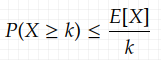
The Markov inequality gives an upper bound on the probability that a non-negative r. v. is greater than or equal to some positive constant (description directly taken from Wikipedia). Usually, it can be used to examine how likely a r. v. can be very large. It is weaker than the Chebyshev’s inequality and requires only the mean. Note that it applies only to r. v. which takes nonnegative values.
According to the Markov’s inequality, for a r. v. X≥0, discrete or continuous
Unlike Markov’s inequality, Chebyshev’s inequality doesn’t require the r. v. to be non-negative. And it requires not only the mean but also the variance. This inequality bounds the probability that the r. v. is far from the it’s mean:
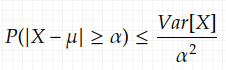
which can be proved using the Markov’s inequality.
The Borel-Cantelli lemma
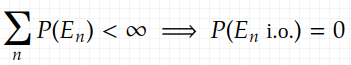
The Borel-Cantelli lemma says that
for any sequence of events {E_n} (a quick note that those E_n’s are sets, which are elements of some σ-field), if the sum of the probabilities of the events {E_n} is finite, then the probability that infinitely many of them occur is 0. Formally
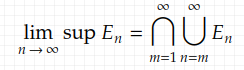
Here “i.o.” stands for “infinitely often”, meaning that event E_n can happen for infinitely many n. E_n i.o. is a more intuitive version of the limit superior:
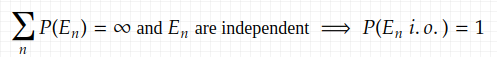
Note that there’s no requirement for independence in this lemma. But the second Borel-Cantelli lemma does require independence, which states
if the sum of the probabilities of the events {E_n}, which are independent, diverges to infinity, then the probability that infinitely many of them occur is 1. Formally
It might not be clear why E_n i.o. and (1.1) are the same thing. So lets have a close look at it. Simply expanding (1.1) gives us

Consider an element from the sample space s, that belongs to this limit superior (it’s also a set of course). And no matter how far you go in the sequence, you will encounter such a set, where n is arbitrarily large:
and s belongs to this set.
Let’s use the favorite example in probability — a coin toss. Consider the infinite coin toss case, and let E_0 be the event that you see a head right away, that would be a set of sequences starting with “H”; let E_1 be the event that a head occurs after one tail…etc. Those events look roughly as follows
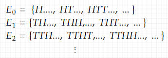
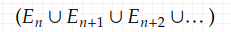
And the limit superior of this sequence of events is that you never see a head. Using the Borel-Cantelli lemma we introduced before, we can easily see that this event has a probability of zero. The sum of those events E_n is
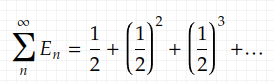
where the first term is the probability that you see head right at the first toss, which is 1/2, as easy as that since we don’t need to consider any following outcomes after the first toss because this coin tossing sequence is memory-less. The second term is the probability that you see a head at the second toss, which only requires that the first toss is T and the second is H. This gives (1/2)². Similarly, the third term is the probability that you see a head at the third toss, which only requires the first three tosses to take on a certain value. This gives (1/2)². We can see that this is a geometric sequence with a common ratio between adjacent items <1. (1.2) evaluates to
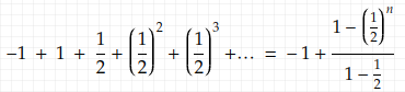
(that -1+1 is there so that we can use the formula of the summation of the geometric sequence) as n goes to infinity, (1.2) converges to 1 < ∞.
This means E_n can not happen for infinitely many n, though it’s true that E_n can happen for an arbitrarily large amount of n (Think about the difference between ∞ and large numbers). In this concrete example, “E_n cannot happen for infinitely many n” means the event E_n containing sequences with infinitely many leading “T” happens with probability 0.
Here is another example that uses the second Borel-Cantelli lemma to show another fact about infinite coin toss. If we toss a fair coin infinitely many times, the head will occur infinitely often. In this case, the events E_n’s are independent coin tosses where you see a head. This is much more straightforward than the previous example. The sum of the probability of those events is
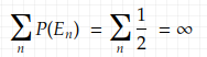
which is just a sum of a constant and diverges. This event E_n — toss a head, happens for infinitely many n, i.e. infinitely often.
The weak law of large numbers(WLLN) & convergence in probability
Let’s have a look at the formulation of WLLN first:
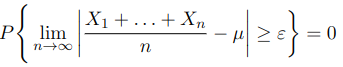
Let X_1, X_2,…, X_n be a sequence of independent identically distributed (i.i.d.) random variables, each having finite mean E[X_i]=μ. Then, for any ε>0,
Note that the sample average
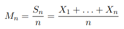
is not a number, but a function, or a r. v. itself. And M_1, M_2,…, M_n is a sequence, whose convergence is of interest. In other words, the WLLN says that the sequence M_1, M_2,…, M_n, or denoted as {M_n} or {S_n/n} for simplicity, converges in probability (later converges in pr. for short). A sequence of r. v. {X_n} converges in probability to a r. v. X is defined as
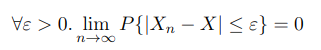
and it is denoted as

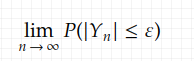
Here is an example of convergence in pr. We consider the following random variable: X_n = X+Y_n, where
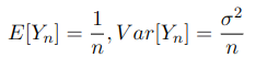
and σ>0 is a constant. It can be directly proved by definition that X_n converges in probability. The approach is rather analytical:
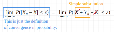
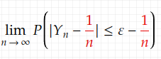
And this leaves us with
It’s an inequality. There are some inequalities we can use. Since in this case, we know the variance, Chebyshev’s inequality can be useful. So now we try to transform (1.3) in such a way that we can apply Chebyshev’s inequality to it. Fortunately, it’s not difficult, we can see that from (1.3) the following also holds, since 1/n>0
Chebyshev’s inequality can be directly used on (1.4) to get an upper bound. Since we know what’s Var[Y_n] already, it’s a simple substitution again:
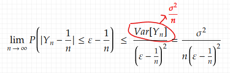
Also, we have (check the order of n, and you can see that it converges to 0)
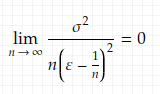
Therefore we have proved (1.4) and can conclude that {X_n} converges in pr.
Sequence {X_n} can also converge to a constant, which can be viewed as a r. v. such that takes on a constant value with probability 1. Here is an example, where the sequence converges in pr. to constant 0:
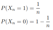
Since we can easily see that
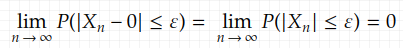
is true because as n goes to infinity, X_n is infinitely close to 0, yet ε is just a fixed constant.
Real-world use case of the convergence of r. v. — The central limit theorem (CLT)
At this point, you might wonder, what’s the point of studying the convergence of a r. v. since in repeating experiments, all the outcomes follow one distribution so the sequence should be i.i.d. But in practice, sometimes it’s not possible to determine the distribution directly, so the convergence of the r. v. is studied instead— we examine to what it approximates.
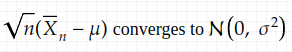
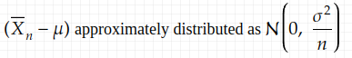
An example of such real-life application of convergence of r. v. is the central limit theorem (CLT), a theorem that connects probability and statistics. Remember we have just mentioned that the sample mean itself is a r. v. So it follows some probability distribution, and what is it? It’s hard to say. Therefore, the convergence of it is studied. According to the CLT, for a sample size n, which is large enough, the distribution approximates the normal distribution 𝓝(μ, σ²/n) (Here the variance depends on n and can’t be a limit distribution!), and after normalization the sample mean converges to 𝓝(0, 1), as n goes to infinity. Formally,
Let X_1, X_2,…,X_n be i.i.d. r. v. with expected value E[X_i]=μ < ∞ and variable 0 < Var[X_i]=σ²< ∞. Then the normalized r. v.
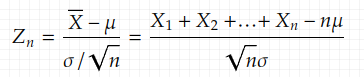
converges in distribution to the standard normal distribution as n, the sample size, goes to infinity. That is
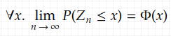
where Φ(x) is the cumulative distribution of the normal distribution.
Convergence in distribution won’t be discussed in depth in this post, just keep in mind that convergence in pr. implies convergence in distribution. (And yes, there is an even weaker form of convergence of r. v. than convergence in pr.)
So far that’s all for the CLT, there will be further discussion about the relationship between the LLN and CLT at the end of this post.:)
The strong law of the large numbers (SLLN) & convergence almost surely
The formulation of the SLLN is seemingly very similar to the weak version with the same requirements of the r. v. X_i:
Let X_1, X_2,…,X_n be a sequence of i.i.d. r. v., each having finite mean E[X_i]=μ. Then
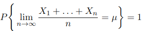
This means that the probability that the sample mean converges to the real mean μ is 1. The probability of this event, the probability of the convergence of the sample mean, is either 0 or 1. The follows Kolmogorov’s zero-one law, which says that the probability of the limit superior is either 0 or 1, in the setting of the 2nd Borel-Cantelli lemma. This is another big topic worth diving into, let’s save it for another post.:)
SLLN states something stronger about the convergence of the sequence {S_n} — it converges almost surely (later a.s. for short). When something happens almost surely, it happens with probability 1. Almost sure convergence for a sequence of r. v. {X_n} is formulated as
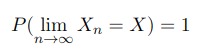
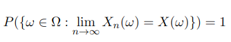
Or more rigorously using the probability space (Ω, 𝓕, P)
You can also see a similar short-form “a.e”., which means “almost everywhere”. The only difference is that they are used in different contexts. You usually see a.e. in measure theory and a.s. in probability theory. But just like “probability” and “measure”, sometimes they are the same thing.
Convergence in pr. vs. convergence a.s.
Since essentially, both laws of large numbers are about the convergence of the sample mean, convergence in probability and almost sure convergence will be discussed first here. We know that convergence in pr. is weaker, so convergence a.s. implies convergence in pr. but not vice versa. A well-known example of sequence {X_n} which converges in probability but doesn’t converge a.s. is the example we have seen in the previous section. Let’s revisit example (2.1):
Not that those X_i’s are mutually independent but not with identical distributions. All of them satisfy the Bernoulli distribution but with different parameters. An example of i.i.d. r. v. will be used later to demonstrate how is WLLN weaker.
Why doesn’t {X_n} converge a.s.? It’s not a difficult question to answer now since we are already equipped with the Borel-Cantelli lemma. The sum of the probability of the events X_n = 1 is
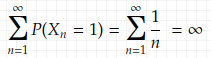
which is the sum of a harmonic sequence. It’s an important fact in real analysis that it’s a divergent sequence. Therefore, according to the second Borel-Cantelli lemma and combined with the definition of almost sure convergence (4.1), {X_n} doesn’t converge almost surely.
From what has been discussed so far, the subtle difference between convergence in pr. and convergence a.s. can be concluded as follows:
In both cases, convergence in pr. or a.s., outliers can occur, but convergence in pr. doesn’t specify how often they happen, but convergence a.s. yes, it says that outliers can occur only finitely many times.
WLLN vs. SLLN
Both of the laws of large numbers show that, in an experiment, as sample size n goes to infinity, the average of the outcome from the samples gets to be very close to the population mean. But the difference between them lies in the difference between the two different types of convergences, which is mentioned at the end of the last section.
One thing that can seem to be strange is that since the conditions of both laws are the same, the weaker conclusion seems redundant. (Under the same condition, we know that B is valid, which covers A, why would we need to state A anyway?) Here is a note on those conditions: The aforementioned conditions for both laws are the same, but they differ in necessities. The SLLN requires a finite mean (E[X_i] < ∞), but the WLLN can be proved without this. Therefore, when an example of a distribution, for which the WLLN holds but the SLLN doesn’t, is demonstrated, the condition of the finite mean is relaxed.
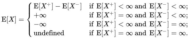
Here “finite mean” is mentioned, which brings up an important note that a random variable can have an “infinite mean” when the mean “doesn’t exist”, that’s a different situation. We have the following possible situations:
On Wikipedia, examples of probability distributions, for which the WLLN holds but SLLN does not, are given. There’s not much explanation, but now it makes much more sense. Here is the first example on Wiki:
Let X be an exponentially distributed r. v. with parameter 1, which means the probability density function is
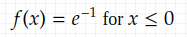
and f(x)=0 for x<0. Then the r. v.
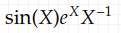
has no expected value. Why? We can see that using the conditional divergence of (6.1) and by definition of the expected value
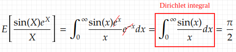
the sum above is not absolute convergent, though it converges in pr. and WLLN holds. The Dirichlet integral is Riemann integrable and evaluates to π/2, and the sample mean converges in pr. to this, but

is not even Lebesgue integrable due to the failure of absolute convergence. (Lebesgue integration is more general than Riemann integration.) For a visualization of how this fails in simulated sampling, see here.
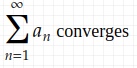
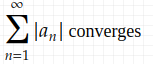
Here is a quick reminder of the definition of absolute convergence and conditional convergence: Given a sequence {a_n}, we say that the sum of {a_n}
- converges absolutely, if
- converges conditionally, if
We need absolute convergence to make the expected value make sense, meaning that the definition of r. v. with probability mass (analogical for probability density) reads
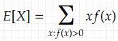
whenever this sum is absolutely convergent.
That’s because the expected value should not depend on the order of the outputs, and for a conditionally convergent sequence, you can shuffle the whole sequence and make it converge to anything (though permuting finite many of them doesn’t make much difference).
How about SLLN, when there’s no finite mean or no mean at all? According to the theorem in [2], if X_i does not have a finite mean, then S_n/n almost surely diverges, which means one of the following situations will occur:
1. P{lim(S_n/n) = +∞} = 1.
2. P{lim(S_n/n) = -∞} = 1.
3. P{lim sup(S_n/n) = +∞ and lim inf{S_n/n} = -∞} = 1.
as n goes to infinity.
Sometimes you can see the requirement of finite variance for both LLNs, but that’s not necessary for either of them. It’s for the ease of proof.
The differences between the SLLN and the WLLN are rather theoretical since in real life we don’t very often deal with infinity and computers just can’t handle it. According to this, there don’t seem to be any examples where the distinction between the WLLN and the SLLN makes any difference.
Relationship between the LLN and the CLT — revisit the CLT
After knowing so much about the LLN, here comes the great moment to revisit the CLT and close this post. It might seem weird at first glance that the LLN says that the central mean converges to the population mean, which is a constant, in the mean while the CLT says that the sample mean converges to the normal distribution. But in fact, there is no contradiction at all.
The confusion is mostly due to the difference between
and
two pieces of information conveyed in the CLT. If we look at 𝓝(μ, σ²/n) in (7.2), as n goes to infinity, the variance of the sample mean goes to 0, which means the graph of the normal distribution becomes narrower and narrower, until it concentrates at 0 and becomes a degenerate function. In this case, the probability mass concentrates at the event that the sample mean is μ, the population mean, which is similar to what LLN states.
And (7.1) tells us the same thing, but dividing by the square root of the sample size rescales the shape so that the normal distribution doesn’t degenerate.
What CLT tells us more than LLN is how the sample mean goes towards the population mean, as sample size grows. So does CLT contain LLN? Logically not really, since CLT requires finite variance but LLN doesn’t, LLN can be used for more occasions, which makes LLN more powerful.
Conclusion
The main purpose of this post is to help you understand the two versions of LLN in greater depth, and also to connect it with other important statements in probability theory, such as the CLT. We started with the two famous inequalities in probability and the Borel-Cantelli lemma to prepare for the later discussion. Then we moved to the LLN and discovered the differences between the WLLN and the SLLN via the different types of convergence in those LLN. Also, we examined the subtle differences between those two LLNs.
References
[1] Ross, S. M., Ross, S. M., Ross, S. M., & Ross, S. M. (1976). A first course in probability (Vol. 2). New York: Macmillan.
[2]Erickson, K. B. (1973). The strong law of large numbers when the mean is undefined. Transactions of the American Mathematical Society, 185, 371–381.
[3] Pishro-Nik, H. (2014). Introduction to probability, statistics, and random processes (p. 732). Blue Bell, PA, USA: Kappa Research, LLC.


