Dirichlet Distribution: The Underlying Intuition and Python Implementation

Everything you need to know about the Dirichlet distribution

The Dirichlet distribution is a generalization of the beta distribution. In Bayesian statistics, it is commonly used as the conjugate prior to the multinomial distribution, hence it can be used to model the uncertainty of a random vector of probabilities. It has a wide range of applications including Bayesian analysis, text mining, statistical genetics, and nonparametric inference. This article gives an intuitive introduction to Dirichlet distribution and shows how it is connected to the multinomial distribution. In addition, it shows how it can be modeled and visualized in Python.

Definition

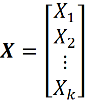
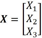
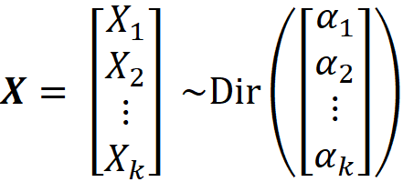
Suppose that the continuous random variables X₁, X₂, …Xₖ (k≥2) form the random vector X defined as:

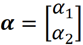
We also define the vector α as:

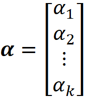
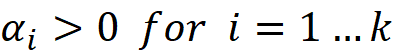
where

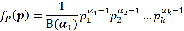
Now the random vector X is said to have Dirichlet distribution with parameter α if it has the following joint PDF:

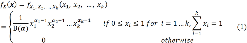
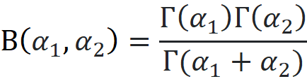
The function B(α) is called the multivariate beta function and is defined as

where Г(x) is the gamma function. If the random vector X has a Dirichlet distribution with parameter α, it is denoted by X ~ Dir(α). The multivariate beta function is included in the joint PDF to normalize it. The joint PDF should integrate to 1 over its domain:

Hence, we have:

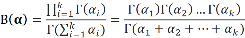
Based on Equation 1, the values that the random variables X₁, X₂, …Xₖ take should meet the following conditions to have fₓ(x)>0:

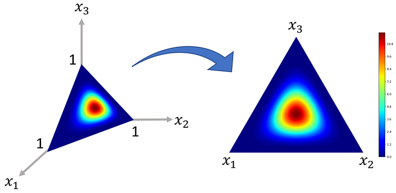
These conditions define the support of the Dirichlet distribution. The support of X, and of its distribution, is the set of all x (the values that X can take) where fₓ(x)>0. If X has k elements, the support of X with a Dirichlet distribution is a k-1 dimensional simplex. A simplex is a bounded linear manifold that is created because of the constraints of Equation 3. A simplex is the generalization of the notion of a triangle to higher dimensions. Hence, a k-1 dimensional simplex can be thought of as a k-1 dimensional triangle which lies in a k-dimensional space.

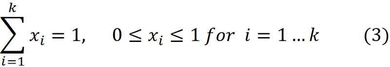
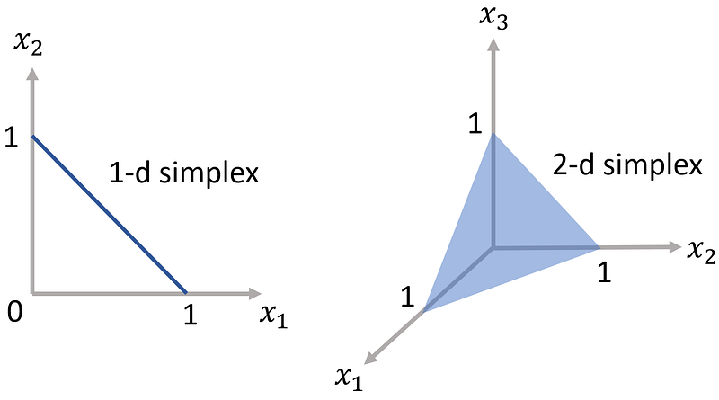
For example, if k=2, then the support of X is the 1-d simplex shown in Figure 1 (left). It is a straight line that touches each axis at a point 1 unit away from the origin. For each point on this line, we have:

For k=3, then the support of X is the 2-d simplex shown in Figure 1 (right). Now it is a triangle that touches each axis at a point 1 unit away from the origin.

For each point on the surface of this triangle, we have:

Let the random vector

has a Dirichlet distribution with the parameter:

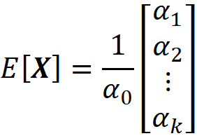
And let

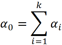
Then, it can be shown that the mean of X is as follows:

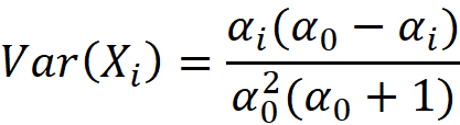
It can be also shown that:

Intuition

As mentioned before, the Dirichlet distribution is commonly used as the conjugate prior for the multinomial distribution. Hence, to understand the intuition behind it, first, we need to review the multinomial distribution. Suppose that the discrete random vector X is defined as:

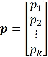
And let the vector p be:

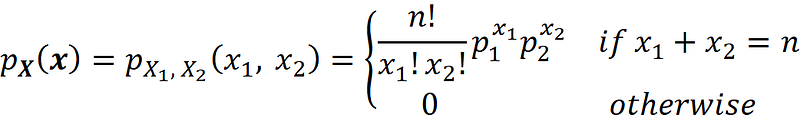
Then X is said to have the multinomial distribution with parameters n and p if it has the following joint PMF:

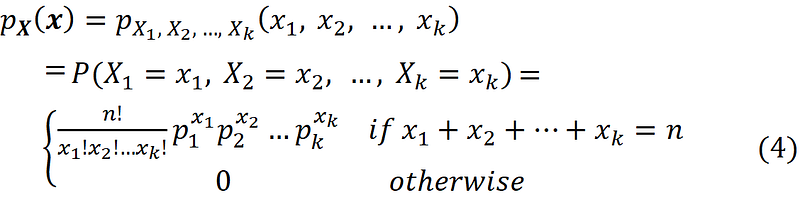
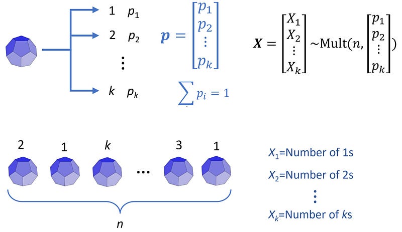
Multinomial distribution can be used to model a k-sided die. Suppose that we have a k-sided die and roll it n times. Let pᵢ denote the probability of getting side i, and let the random variable Xᵢ represent the total number of times that side i is observed (i=1…k). Then the random vector

has a multinomial distribution with parameters n and

This is demonstrated in Figure 2.

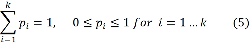
Now suppose that we do not know the values of pᵢ in vector p. Hence, we don’t know the probability of getting each side of the k-sided die, and we want to infer it by observing the outcomes of n rolls of this die. The elements of p represent the probability of some mutually exclusive events, so we should have:

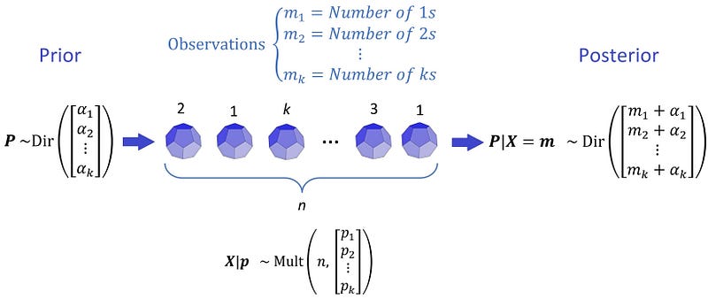
The value of p can be inferred using the Bayesian approach. Here, we assume that the unknown probability vector p is represented by the continuous random vector P. The probability distribution of P is called the prior distribution. The prior distribution represents the prior knowledge or assumptions about the parameter P being estimated. After rolling the die, we can analyze the observed data and use it to update our belief about P. Hence, we end up with a new distribution for P which is called the posterior distribution. The posterior distribution results from updating the prior probability distribution with the observed data.

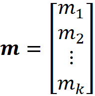
Remember that random variable Xᵢ in the random vector X represents the total number of times that side i is observed. If we know the value of p, we can calculate the probability of observing X₁=m₁, X₂=m₂, …Xₖ=mₖ after n rolls using the following conditional probability:

where:

This conditional gives the probability of observing each side of the die for a specific number of times after n rolls assuming that we know the true value of P. As mentioned before, the probability distribution of P is our prior distribution. We denote the joint PDF of this distribution by f_P(p). Now, we can use Bayes’ rule to connect the prior and posterior joint PDFs:

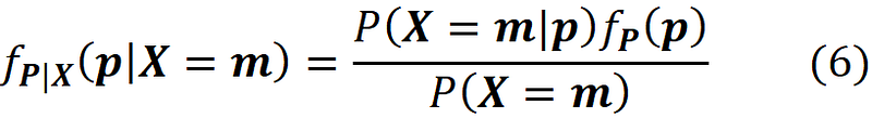
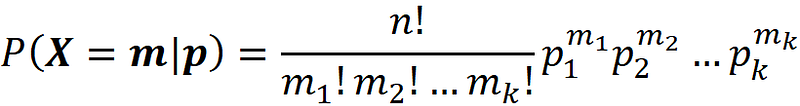
Here f_P|X (p|X=m) is the joint PDF of the posterior distribution. This distribution updates our belief about P after observing X. We also call P(X=m|p) the likelihood, and it can be written as the PMF of a multinomial distribution with a known value of p (Equation 4):

The denominator of Bayes’ rule is the probability of X=m, and it is called the marginal PMF of X:

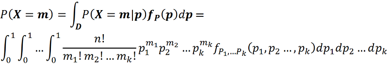
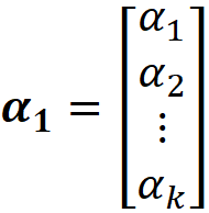
Please note it is independent of the true value of p. Now we assume that the prior distribution is a Dirichlet distribution with the parameter α₁:

where

Remember that the random variables with a Dirichlet distribution should follow the conditions in Equation 3, and these conditions are exactly the same as the conditions of Equation 5. In fact, the conditions in Equation 3 allow us to use the Dirichlet distribution for the random variables that represent the probability of mutually exclusive events.

Now we can use the Bayes’ rule (Equation 6) to write:

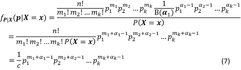
Here c is a constant that does not depend on pᵢ values. The posterior joint PDF should be normalized; hence we have the following condition:

By comparing Equations 7 and 8 with Equations 1 and 2, we conclude that the posterior distribution is a Dirichlet distribution with the parameter

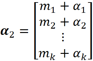
and c is simply its normalizing factor, and we get:

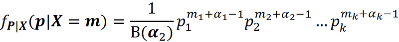
Finally, we can write:

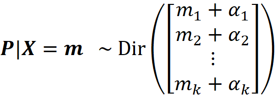
So, if we assume that the prior has a Dirichlet distribution, then the posterior distribution of P after observing X=m is also a Dirichlet distribution. We only need to add the observed number of each side (mᵢ) to its corresponding parameter in the prior distribution (αᵢ) to get the parameters of the posterior distribution.

In Bayesian probability theory, If the posterior distribution belongs to the same family as the prior distribution, then the prior and posterior are referred to as conjugate distributions. Therefore, we conclude that the Dirichlet distribution is the conjugate prior to the multinomial distribution (Figure 3).

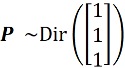
One special case of the Dirichlet distribution is when

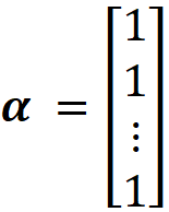
Then we have:

which means that

is the same as the uniform distribution over its k-1 dimensional simplex since the joint PDF has the same value over the simplex.

Modeling and visualization in Python

We can use the scipy library to model Dirichlet distribution in Python. In scipy, Dirichlet distribution can be created using the object dirichlet. This object takes the parameter alpha which corresponds to α in Equation 1. We can also pass alpha to the methods of this object instead. The method pdf() also takes the parameter x which corresponds to x in Equation 1 and returns the joint PDF of the distribution at x. We can also calculate the mean and variance of the distribution using the methods mean() and var(). For example, let:

Now we want to calculate the mean of X and its joint PDF at [0.5, 0.3, 0.2]ᵀ using the following code snippet:

from scipy.stats import dirichlet
dist = dirichlet([5, 5, 5])
print("PDF at [5,5,5]: ",dist.pdf([0.5, 0.3, 0.2]))
print("Mean of disitrubtion: ", dist.mean())

PDF at [5,5,5]:  5.1081030000000025
Mean of disitrubtion:  [0.33333333 0.33333333 0.33333333]

If the value of x is outside the simplex, pdf() throws an error:

# This results in an error
dist.pdf([0.5, 0.3, 0.3])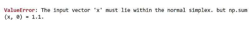

We can visualize the joint PDF of the Dirichlet when k=2 and 3 (k is the number of the elements of X). As mentioned before, when we have 3 random variables in X (with Dirichlet distribution), the simplex is a 2-d triangle (Figure 1). We can calculate the contours of the joint PDF on the surface of this simplex and plot it in a 2-d plot with barycentric coordinates (Figure 4).

The barycentric coordinates are the coordinates of a point with respect to a simplex in an affine space. They can give the location of a point with respect to a line, triangle, or tetrahedron instead of the global Cartesian coordinates. In a k-dimensional Cartesian coordinate system, the coordinates of a point can be expressed as the normalized weighted average of the edges of a k-1 dimensional simplex. Those weights then give the barycentric coordinates of the point relative to that simplex. Consider the 2-d space shown in Figure 5.

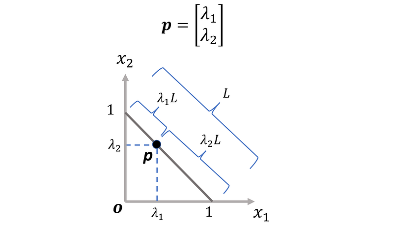
The 1-d simplex is the line segment between the endpoints [0,1] and [0,1]. The coordinates of an arbitrary point p on this simplex can be expressed as the normalized weighted average of coordinates of the endpoints:

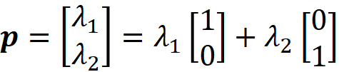
where

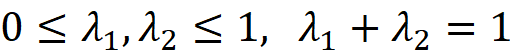
Here λ₁ is the distance of p from the endpoint [0,1] divided by the length of the simplex (L). Similarly, λ₂ is the distance of p from the endpoint [1,0] divided by L. The weights λ₁ and λ₂ are the barycentric coordinates of p relative to this simplex, and since the endpoints are just one unit away from the origin, they have the same values as the Cartesian coordinates.

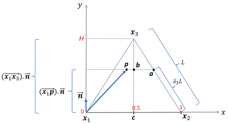
Next, consider the 2-d simplex shown in Figure 6. This simplex is a triangle formed by the endpoints [1,0,0], [0,1,0] and [0,0,1]. The coordinates of a point p on this simplex are equal to the normalized weighted average of the coordinates of these endpoints:

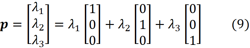
where

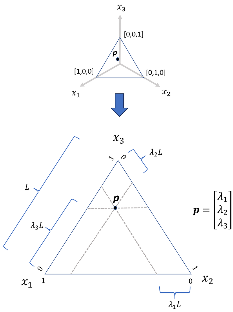
In this triangle, each node represents one of the coordinate axes x₁, x₂, or x₃. Suppose that we want to calculate the value of x₁. Let the length of each side be L (it is an equilateral triangle). To get the value of x₁, we draw a line that passes through p and is parallel to the side that doesn’t pass through the node represented by x₁ (here this side is x₂x₃). This line divides each of the remaining sides (x₁x₂ and x₁x₃) into two segments. On each of these sides, the length of the line segment which does not contain the node x₁ is λ₁L (Figure 6). We can calculate the values of λ₂ and λ₃ similarly.

Now, we create a Python function that draws the contours of the joint PDF of the Dirichlet distribution on a 2-d simplex. Listing 1 imports all the libraries that we need later and defines the edges of this triangular simplex on a 2-d plot. These edges are stored in the list edges. Please note that this 2-d simplex is now plotted on a 2-d screen, hence all the edges are 2-dimensional. However, the barycentric coordinates of a point are still a weighted average of the Cartesian coordinates of these edges:

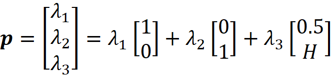
Here H is the height of the triangle (Figure 7).

We use the matplotlib.tri library to create a triangular mesh. The array normal_vecs keeps the normal vectors of each side of this triangle (the normal vector of each side is perpendicular to that side).

# Listing 1

import numpy as np
import matplotlib.pyplot as plt
import matplotlib.tri as tri
from scipy.stats import dirichlet, multinomial, beta
from math import pi
from mpl_toolkits.axes_grid1 import make_axes_locatable
import matplotlib.gridspec as gridspec
%matplotlib inline

H = np.tan(pi/3)*0.5
edges = np.array([[0, 0], [1, 0], [0.5, H]])
shifted_edges = np.roll(edges, 1, axis=0)
triangle = tri.Triangulation(edges[:, 0], edges[:, 1])

# For each edge of the triangle, the pair of other edges
edge_pairs = [edges[np.roll(range(3), -i)[1:]] for i in range(3)]
# The normal vectors for each side of the triangle
normal_vecs = np.array([[pair[0,1] - pair[1,1],
              pair[1,0] - pair[0,0]] for pair in edge_pairs])

In Listing 2, the function cart_to_bc() converts the 2-d Cartesian coordinates of a point into the barycentric coordinates relative to the 2-d triangle defined by the edges in edges.

# Listing 2

def cart_to_bc(coords):
    '''Converts 2D Cartesian coordinates to barycentric'''
    bc_coords = np.sum((np.tile(coords, (3, 1))-shifted_edges)*normal_vecs,
                axis=1) / np.sum((edges-shifted_edges)*normal_vecs, axis=1)
    return np.clip(bc_coords, 1.e-10, 1.0 - 1.e-10)

def bc_to_cart(coords):
    '''Converts barycentric coordinates to 2D Cartesian'''
    return (edges * coords.reshape(-1, 1)).sum(axis=0)  

Figure 7 shows how these calculations are done to calculate λ₃ (as an example). As this figure shows one edge of the triangle (x₁) is at the origin of the 2-d Cartesian coordinate system. We can represent a point p on this triangle with vector x₁p. From geometry, we know that

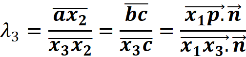
Where n is the normal vector of the side x₁x₂. Hence, if we have the Cartesian coordinates of p, the edges of the triangle, and the normal vector of each side, we can easily calculate the barycentric coordinates of p.

It is important to note that this function doesn’t always return the exact barycentric coordinates. If a barycentric coordinate is outside the interval [1e-10 -10, 1–1e-10], then it is clipped to the interval edges using the clip() function in numpy. The reason for that will be explained later.

We also have the function bc_to_cart() that converts the barycentric coordinates of this triangle to the Cartesian coordinates. The Cartesian coordinates of a point p are equal to the weighted average of the Cartesian coordinates of the edges of the triangle, and the barycentric coordinates are simply the weights:

Finally listing 3 defines the function plot_contours() that draws the contours of the joint PDF of a Dirichlet distribution on this triangle. This function creates a triangular mesh on the Cartesian 2d space. Next, the barycentric coordinates of each point on this mesh are calculated. Then it uses the barycentric coordinates to calculate the joint PDF of that point. After calculating the joint PDF of all the points on the triangle, the contours are plotted. Please note that some points on the triangular mesh can be slightly out of the simple boundary. This means that x₁+x₂+x₃ for that point can be slightly less than zero or greater than 1. Passing such a point to the pdf() method of the dirichlet object throws an error. Hence, we clip the barycentric coordinates in cart_to_bc() to avoid this error.

# Listing 3

def plot_contours(dist, nlevels=200, subdiv=8, ax=None):
    refiner = tri.UniformTriRefiner(triangle)
    mesh = refiner.refine_triangulation(subdiv=subdiv)
    pdf_vals = [dist.pdf(cart_to_bc(coords)) for coords in zip(mesh.x, mesh.y)]
    if ax:
        contours = ax.tricontourf(mesh, pdf_vals, nlevels, cmap='jet')
        ax.set_aspect('equal')
        ax.set_xlim(0, 1)
        ax.set_ylim(0, H)
        ax.set_axis_off()
    else:
        contours = plt.tricontourf(mesh, pdf_vals, nlevels, cmap='jet')
        plt.axis('equal')
        plt.xlim(0, 1)
        plt.ylim(0, H)
        plt.axis('off')
    return contours

Let's try plot_contours(). We first plot the contours of

As mentioned before, it is the same as the uniform distribution over its 2-d simplex since the joint PDF has the same value over the simplex. Listing 4 plots the contours of the joint PDF, and the resulting plot is shown in Figure 8.

# Listing 4

plt.figure(figsize=(10, 10))
contours = plot_contours(dirichlet([1, 1, 1]))
v = np.linspace(0, 3, 2, endpoint=True)
plt.colorbar(contours, ticks=[1,2,3], fraction=0.04, pad=0.1)
plt.text(0-0.02, -0.05, "$p_1$", fontsize=22)
plt.text(1-0.02, -0.05, "$p_2$", fontsize=22)
plt.text(0.5-0.02, H+0.03, "$p_3$", fontsize=22)
plt.title("Dir([1,1,1])", fontsize=22)
plt.show()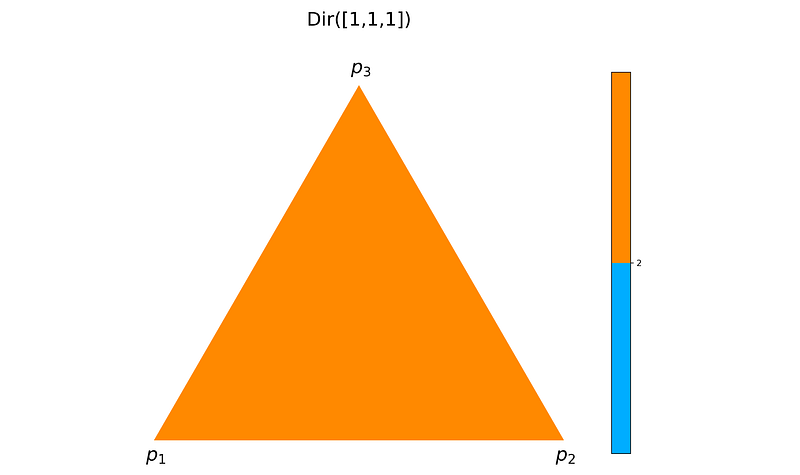

As you see the joint PDF has the same value all over the simplex. Next, we plot the contours of

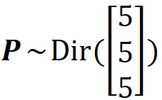
as our second example in Listing 5. The result is shown in Figure 9.

# Listing 5

plt.figure(figsize=(10, 10))
contours = plot_contours(dirichlet([5, 5, 5]))
plt.colorbar(contours, fraction=0.04, pad=0.1)
plt.text(0-0.02, -0.05, "$p_1$", fontsize=22)
plt.text(1-0.02, -0.05, "$p_2$", fontsize=22)
plt.text(0.5-0.02, H+0.03, "$p_3$", fontsize=22)
plt.title("Dir([5,5,5])", fontsize=22)
plt.show()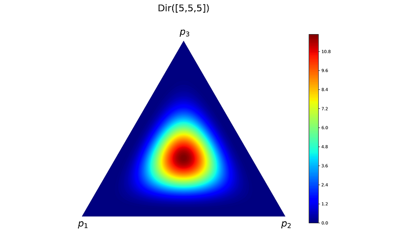

Effect of α on the joint PDF

We can also create a 3d plot of the surface of the joint PDF. Here we assume that the 2-d simplex is on the XY plane and the Z axis gives the value of the PDF. The function plot_surface() in Listing 6 generates such a plot.

# Listing 6

def plot_surface(dist, ax, nlevels=200, subdiv=8, log_plot=False, **args):
    refiner = tri.UniformTriRefiner(triangle)
    mesh = refiner.refine_triangulation(subdiv=subdiv)
    pdf_vals = [dist.pdf(cart_to_bc(coords)) for coords in zip(mesh.x, mesh.y)]
    pdf_vals = np.array(pdf_vals, dtype='float64')
    if log_plot:
        pdf_vals = np.log(pdf_vals)
    ax.plot_trisurf(mesh.x, mesh.y, pdf_vals, linewidth=1, **args)

Listing 7 uses this function to plot the joint PDF of the Dirichlet distribution with some different parameters. The plots are shown in Figure 10.

# Listing 7

fig = plt.figure(figsize=(15, 10))
ax1 = fig.add_subplot(231, projection='3d')
ax2 = fig.add_subplot(232, projection='3d')
ax3 = fig.add_subplot(233, projection='3d')
ax4 = fig.add_subplot(234, projection='3d')
ax5 = fig.add_subplot(235, projection='3d')
ax6 = fig.add_subplot(236, projection='3d')

ax = [ax1, ax2, ax3, ax4, ax5, ax6]
params = [[1,1,1], [1,7,1], [0.65,7,1], [5,5,5], [30,30,30], [5, 5, 30]]

for i in range(6):
    plot_surface(dirichlet(params[i]), ax[i],
                 antialiased=False, color='yellow')
    ax[i].view_init(35, -135)
    ax[i].set_title("Dir({})".format(params[i]), fontsize=16)
    ax[i].zaxis.set_rotate_label(False) 
    ax[i].set_zlabel("$f_\mathregular{P}(\mathregular{p})$", fontsize=16,
                     weight="bold", style="italic", labelpad=5, rotation=90)
    ax[i].set_xlim([-0.15, 1.1])
    ax[i].set_ylim([-0.15, 1.1])
    if i>2:
        ax[i].set_zlim([0, 65])
    ax[i].xaxis.set_ticklabels([])
    ax[i].yaxis.set_ticklabels([])
    ax[i].set_xticks([])
    ax[i].set_yticks([])
    if i==0:
        ax[i].text(-0.15, -0.07, 2, "$p_1$", fontsize=14)
        ax[i].text(1.07, 0.03, 2, "$p_2$", fontsize=14)
        ax[i].text(0.5, H+0.15, 2, "$p_3$", fontsize=14)
    else:
        ax[i].text(-0.15, -0.07, 0, "$p_1$", fontsize=14)
        ax[i].text(1.07, 0.03, 0, "$p_2$", fontsize=14)
        ax[i].text(0.5, H+0.15, 0, "$p_3$", fontsize=14)

plt.show()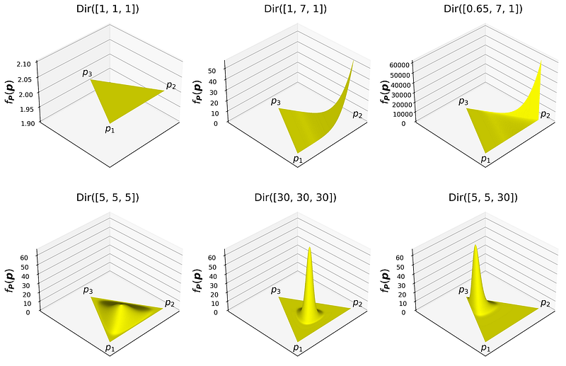

These plots can help you understand the effect of α on the shape of the joint PDF. The random variables p₁, p₂, and p₃ in P with a Dirichlet distribution can represent the probability of 3 mutually exclusive events. Hence, each edge of the simplex represents one of these events, and the corresponding αᵢ is like a weight for the likelihood of that event.

As mentioned before α=[1 1 1]ᵀ means that we have a uniform distribution over the simplex. Here, the value of PDF is 2 everywhere over the simplex, so the joint PDF has a flat surface. When αᵢ increases relative to other elements, it means that the ith event has a higher chance of occurrence since it has been observed more compared to other events (here we can assume that we start we Dir([1 1 1]ᵀ) as the prior distribution). An example is the plot of Dir([1 7 1]ᵀ) in Figure 10. Now the surface is raised near the edge of the simplex that represents that event.

When the sum α₁+α₂+α₃ increases, it means that the total number of observations has increased. This will decrease our uncertainty about the distribution of P and makes the joint PDF of the Dirichlet distribution look shaper. As you see in Figure 10, Dir([30 30 30]ᵀ) is much sharper compared to Dir([5 5 5]ᵀ). However, both look symmetric with respect to edges. Since all the events have been observed equally. When an αᵢ gets larger compared to others, the peak of the joint PDF moves towards the edge representing it. This is shown in Dir([5 5 30]ᵀ). Here the weight of the 3rd event (α₃) is greater which means that the 3rd event has been observed more, so it has a higher chance of occurrence.

Please note that all the elements of α should be greater than zero, so we can not assign a zero weight to an event. However, if we set αᵢ<1 then, the weight of the corresponding event significantly drops. This is shown in the plot of Dir([0.65 7 1]ᵀ) in Figure 10. If you compare it with the plot of Dir([1 7 1]ᵀ), you see that to have a nonzero PDF, the barycentric coordinate of p₁ should be very small. This is almost like having a 1-d simplex on p₂ and p₃.

Listing 8 plots the joint PDF of the Dirichlet distribution on a logarithmic scale (to better show the changes of the joint PDF surface). The result is shown in Figure 11.

# Listing 8

fig = plt.figure(figsize=(15, 10))

ax1 = fig.add_subplot(121, projection='3d')
ax2 = fig.add_subplot(122, projection='3d')

ax = [ax1, ax2]
params = [[0.2, 0.2, 0.2], [0.8,0.8,0.8], [0.2,0.5,1]]

for i in range(2):
    plot_surface(dirichlet(params[i]), ax[i], log_plot=True, cmap='jet')
    ax[i].view_init(10, -135)
    ax[i].set_title("Dir({})".format(params[i]), fontsize=20)
    ax[i].zaxis.set_rotate_label(False) 
    ax[i].set_zlabel("$log(f_\mathregular{P}(\mathregular{p}))$",
                     fontsize=18, weight="bold", style="italic",
                     labelpad=5, rotation=90)
    ax[i].set_xlim([-0.15, 1.1])
    ax[i].set_ylim([-0.15, 1.1])
    ax[i].set_zlim([0, 17])
    ax[i].xaxis.set_ticklabels([])
    ax[i].yaxis.set_ticklabels([])
    ax[i].set_xticks([])
    ax[i].set_yticks([])
    ax[i].text(-0.09, -0.07, 0, "$p_1$", fontsize=14)
    ax[i].text(1.07, 0.03, 0, "$p_2$", fontsize=14)
    ax[i].text(0.5, H+0.22, 0, "$p_3$", fontsize=14)

plt.show()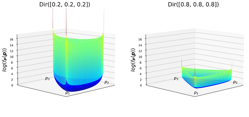

Note that when all αᵢ are less than 1, the joint PDF has a convex surface. The PDF is extremely small except at the edges and the sides of the triangular simplex. It is almost like having three 1-d simplexes at the sides of the triangle. Hence a prior with such a distribution represents a setup in which one or two pᵢ are extremely small, and their corresponding events have a small chance of occurrence.

By comparing Dir([0.2 0.2 0.2]ᵀ) with Dir([0.8 0.8 0.8]ᵀ), you notice that increasing the value of αᵢ tends to flatten the surface of the joint PDF. Hence, it decreases the value of the joint PDF on the edges and sides and increases its value in the regions closer to the middle of the simplex.

Finally, it is important to note that the parameters of the Dirichlet distribution can be also non-integers. But what is the meaning of say Dir([1.65 6 20]ᵀ)? Here, we can assign the fractional part of the parameters to the prior distribution. For example, we can write it as Dir([0.65+1 1+5 7+13]ᵀ). This means that we started with Dir([0.65 1 7]ᵀ) as the prior distribution (the joint PDF of Dir([0.65 1 7]ᵀ) is shown in Figure 10). Choosing this prior distribution means that we initially believed that p₁ is almost zero, and its corresponding event is very unlikely to happen. Then we observed that the 1st event occurred only once, and the 2nd and 3rd events event occurred 5, and 13 times respectively. These numbers were added to the parameters of the prior distribution to form the posterior distribution.

Bayesian inference in Python

Now that we can plot the contours, we can use the Dirichlet distribution to infer the distribution of parameters of a multinomial distribution. Suppose that we have a 3-sided die (of course, it can be also a 6-sided die with only 3 labels (1, 2, and 3) where each label is placed on two faces). Let the probability of getting side i be pᵢ, and Xᵢ represents the total number of times that side i is observed (i=1..3). As mentioned before, the random vector

has a multinomial distribution with parameters n and

Let the actual value of p be:

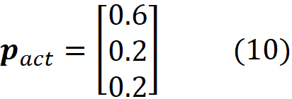
Hence, this is not a fair die! We can use the multinomial object in scipy to model this distribution. The following code snippet shows the result of rolling this die 10 times:

p_act = np.array([0.6, 0.2, 0.2])
sample = multinomial.rvs(n=10, p=p_act, random_state=1)
sample

array([6, 3, 1])

Hence if we roll it 10 times, we have the following observation:

• Side 1: 6 times
• Side 2: 3 times
• Side 3: only 1 time

Of course, these are some random events, so if we change the random_state in rvs() , we can get a different observation (we fix the random_state to make this specific observation repeatable).

Now suppose that we don’t have the probability of getting each side, so the actual value of the vector p (which was given in Equation 10) is unknown. However, we can still roll this die n times and observe the outcomes, therefore, we know the values of Xᵢ. If we assume that the unknown probability vector p is represented by the random vector P, we can use the Dirichlet distribution to infer the probability distribution of P after rolling the die.

Listing 9 first generates the outcomes of rolling the die n times and stores it in m. Then it calculates f_P|X (p|X=m) which is the joint PDF of the posterior distribution and plots its contours on a 2-d simplex. We have tried 5 different values for n ranging from 3 to 10000, and the plots are shown in Figure 12. We start with Dir([1 1 1]ᵀ) as the prior distribution for P. So initially we have a uniform distribution for P in which different values of P are equally likely. Hence, we have the maximum uncertainty about P.

The actual value of P (Equation 10) which was used to generate the observation data is shown with a white marker on these plots. As n increases, we get more observation data, and our uncertainty about P decreases. By increasing n, the Dirichlet distribution, which was initially uniform, gets sharper and closer to the white market that represents p_act.

# Listing 9

p_act_coords = bc_to_cart(p_act)

alpha_prior = [1, 1, 1]
number_rolls = [3, 15, 50, 500, 10000]
num_cols = 2

fig, axes = plt.subplots(3, num_cols, figsize=(16, 25))
plt.subplots_adjust(wspace=0.2, hspace=0.05)

contours = plot_contours(dirichlet(alpha_prior), ax=axes[0, 0])
axes[0, 0].set_title("Prior distribution", fontsize=22, pad=50)
axes[0, 0].scatter(p_act_coords[0],
                   p_act_coords[1],
                   s=300, color='white',
                   marker='+')
axes[0, 0].text(0-0.02, -0.05, "$p_1$", fontsize=16)
axes[0, 0].text(1-0.02, -0.05, "$p_2$", fontsize=16)
axes[0, 0].text(0.5-0.02, H+0.05, "$p_3$", fontsize=16)
divider = make_axes_locatable(axes[0, 0])
cax = divider.append_axes('right', size='2%', pad=0.2)
cbar = fig.colorbar(contours, cax=cax)

for i in range(1, 6):
    m= multinomial.rvs(n=number_rolls[i-1], p=p_act, random_state=0)
    contours = plot_contours(dirichlet(m + alpha_prior),
                             ax=axes[i // num_cols, i % num_cols])
    axes[i//num_cols, i%num_cols].set_title("n={}".format(number_rolls[i-1]),
                                            fontsize=22, pad=50)
    axes[i//num_cols, i%num_cols].scatter(p_act_coords[0],
                                          p_act_coords[1],
                                          s=300, color='white',
                                          marker='+')
    axes[i//num_cols, i%num_cols].text(0-0.02, -0.05,
                                       "$p_1$", fontsize=16)
    axes[i//num_cols, i%num_cols].text(1-0.02, -0.05,
                                         "$p_2$", fontsize=16)
    axes[i//num_cols, i%num_cols].text(0.5-0.02, H+0.05,
                                         "$p_3$", fontsize=16)
    divider = make_axes_locatable(axes[i // num_cols, i % num_cols])
    cax = divider.append_axes('right', size='2%', pad=0.2)
    cbar = fig.colorbar(contours, cax=cax)

plt.show()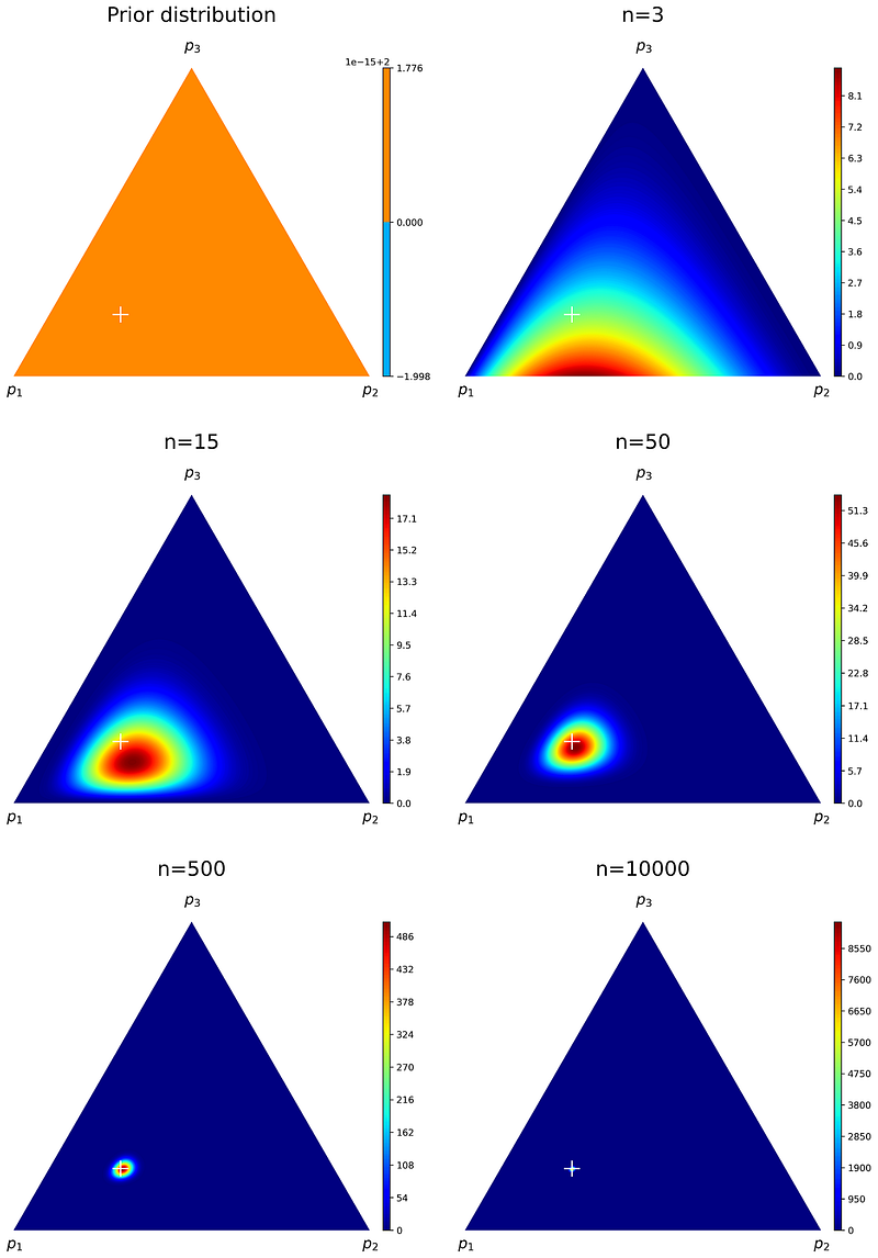

Relation to beta distribution

Let the random vector

have a Dirichlet distribution with the parameter

Based on Equation 1, the joint PDF of X is:

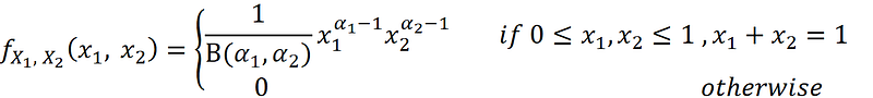
where

Since we have

We can remove x₂ from the PDF:

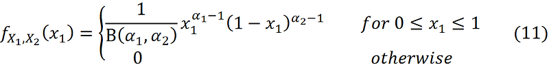
As you see the joint PDF of X₁ and X₂ is only a function of x₁. Hence, the random vector X is determined by the single random variable X₁ which means that the right-hand side of the above equation is also the PDF of the random variable X₁. So, we can write:

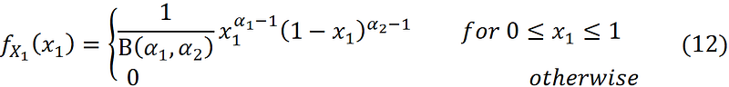
A continuous random variable with such a PDF is said to have the beta distribution with parameters α₁ and α₂, and we denote it by X₁ ~ Beta(α₁, α₂). Similarly, we can write the PDF in terms of x₂:

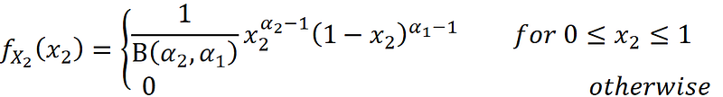
Hence, we conclude that X₂ ~ Beta(α₂, α₁), and we conclude that:

The distributions of X₁ and X₂ are called the marginal distributions of X. The beta distribution is a special case of the Dirichlet distribution when α only has two elements and we only consider one of the random variables in X. Hence it is a univariate distribution. Listing 10 plots the joint PDF of Dir([5 1]ᵀ) and the PDF of its marginal distributions: Beta(5,1) and Beta(1,5). The plots are shown in Figure 13.

# Listing 10

N = 1000
simplex_edges = np.array([[1,0], [0,1]])
tol=1e-6
gamma1 = np.linspace(tol, 1-tol, N)
gamma2 = 1-gamma1
bc_coords = np.stack((gamma1, gamma2), axis=-1)
cart_coords = gamma1.reshape(-1,1)*simplex_edges[0] + \
              gamma2.reshape(-1,1)*simplex_edges[1]
alpha = [5, 1]
pdf = [dirichlet(alpha).pdf(x) for x in bc_coords]

x = np.arange(0, 1.01, 0.01)
param_list = [(1,1), (2,2), (5,1)]
beta_dist1 = beta.pdf(x=x, a=alpha[0], b=alpha[1])
beta_dist2 = beta.pdf(x=x, a=alpha[1], b=alpha[0])

fig = plt.figure(figsize=(15, 15))
plt.subplots_adjust(wspace=0.2, hspace=0.1)
gs = gridspec.GridSpec(2, 2, width_ratios=[2.5, 1],
                       height_ratios=[1, 2.5])
ax1 = fig.add_subplot(221, projection='3d')
ax2 = fig.add_subplot(222)
ax3 = fig.add_subplot(223)

ax1.plot(simplex_edges[:,0], simplex_edges[:,1],
         [0,0], color = 'gray', label='1-d Simplex')
ax1.plot(cart_coords[:,0], cart_coords[:,1], pdf, color = 'black',
         label='Dir([{},{}])'.format(alpha[0], alpha[1]))
ax1.plot(x, [0]*len(x), beta_dist1, color = 'blue',
         label='Beta({},{})'.format(alpha[0], alpha[1]))
ax1.plot([0]*len(x), x, beta_dist2, color = 'green',
         label='Beta({},{})'.format(alpha[1], alpha[0]))

ax1.view_init(25, -135)
ax1.set_xlabel("$x_1$", fontsize=18)
ax1.set_ylabel("$x_2$", fontsize=18, labelpad= 9)
ax1.set_zlabel("$f_\mathregular{X}(\mathregular{x})$", fontsize=18,
               weight="bold", style="italic",
               labelpad= 2, rotation = 45)
ax1.set_xlim([0, 1])
ax1.set_ylim([0, 1])
ax1.set_zlim([0, 6])
ax1.grid(False)
ax1.legend(loc='best', fontsize= 14)

ax2.plot(x, beta_dist1, label='Beta({},{})'.format(alpha[0],
         alpha[1]), linewidth=2, color='blue')
ax2.set_xlabel('$x_1$', fontsize=18)
ax2.set_ylabel('$f_{X_1}(x_1)$', fontsize=18)
ax2.legend(loc='upper left', fontsize= 16)
ax2.set_xlim([0,1])
ax2.tick_params(axis='both', which='major', labelsize=12)

ax3.plot(x, beta_dist2, label='Beta({},{})'.format(alpha[0],
         alpha[1]), linewidth=2, color='blue')
ax3.set_xlabel('$x_2$', fontsize=18)
ax3.set_ylabel('$f_{X_2}(x_2)$', fontsize=18)
ax3.legend(loc='upper right', fontsize= 16)
ax3.set_xlim([0,1])
ax3.tick_params(axis='both', which='major', labelsize=12)
plt.show()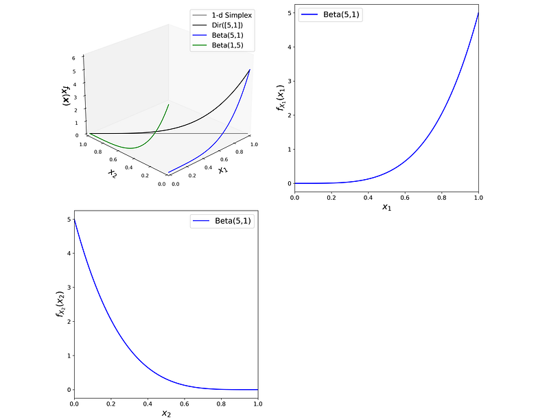

Please note that the joint PDF of Dir([α₁ α₂]ᵀ) in Equation 11 is the same as the PDF of its marginal distribution (Beta(α₁, α₂)) in Equation 12. However, they don’t represent the same distributions. The former is the joint PDF of the random vector X and the latter is the PDF of the random variable X₁. As Figure 13 shows the PDFs of the marginal distributions are the projection of the joint PDF on the planes formed by the axes (x₁, fₓ(x)), and (x₂, fₓ(x)).

Remember that the multinomial distribution can be used to model a k-sided die. When k=2, the die turns into a coin. Now X₁ can represent the total number of heads in n tosses of this coin. Similarly, X₂ represents the total number of tails. From Equation 4, we have:

Since x₁+x₂=n, p₁+p₂=1, we can eliminate p₂ and x₂ from the above equation:

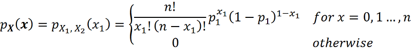
Now the random vector X is determined by the single random variable X₁ which means that the right-hand side of the above equation is also the PDF of the random variable X₁. Hence the PDF of X₁ can be written as:

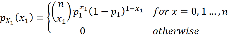
This is the PDF of the binomial distribution. The binomial distribution is a special case of the multinomial distribution when the random vector X has only one element (it is the marginal distribution of the multinomial distribution). Hence X₁ has a binomial distribution with parameters n and p₁. Similarly, X₂ has a binomial distribution with parameters n and p₂.

Since the beta and binomial distributions are special cases of Dirichlet and multinomial distributions respectively, they are still conjugate distributions. In fact, the beta distribution is the conjugate prior to the binomial distribution as shown in Figure 14.

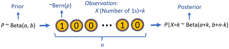
Suppose that we have a coin that lands on heads with an unknown probability of p. Let the random variable P represents the unknown probability p, and the random variable X represents the total number of heads in n tosses. Let’s assume that the probability distribution of P is Beta(a, b) (this is our prior distribution). Now if we toss the coin n times and we observe that X=k, the posterior distribution of P is Beta(a+k, b+n-k).

Aggregation property

Let the random vector X have the following Dirichlet distribution:

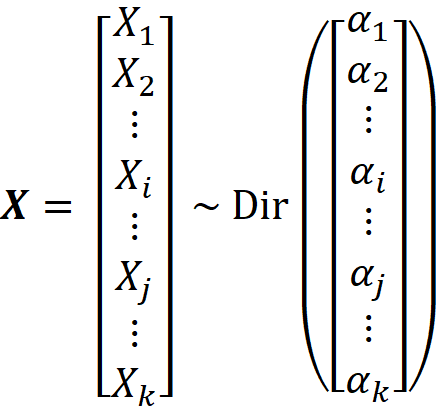
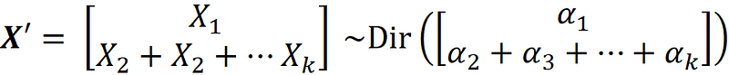
We drop the random variables Xᵢ and X_j from X and add Xᵢ+X_j to it at an arbitrary place and call the resulting random vector X’. It can be shown that X’ has the following Dirichlet distribution:

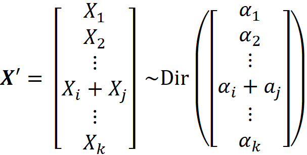
So, to create the vector of parameters in the new Dirichlet distribution, first, we drop the corresponding parameters of Xᵢ and X_j (αᵢ and α_j), and then insert αᵢ+α_j at the same place that Xᵢ +X_j was inserted into X (the index of αᵢ+α_j and Xᵢ +X_j are the same in their corresponding vectors). The proof of the aggregation property is given in the appendix.

Let’s see an example. Let X ~ Dir([1 5 3]ᵀ). Using the aggregation property, we have:

Listing 11 plots the joint PDF of all these distributions together. The plot is in Figure 15. In this plot, each aggregated random vector [Xᵢ X_j+X_k]ᵀ has 1-d simplex. Here, we assumed that this simplex is along the height of the triangle that passes through Xᵢ.

# Listing 11

N = 1000
alpha = [1, 5, 3]

edges_marg_x1 = np.array([[0,0], [0.75,0.5*np.cos(pi/6)]])
edges_marg_x2 = np.array([[1,0], [0.25,0.5*np.cos(pi/6)]])
edges_marg_x3 = np.array([[0.5,H], [0.5,0]])
tol=1e-6
gamma1 = np.linspace(tol, 1-tol, N)
gamma2 = 1-gamma1
bc_coords = np.stack((gamma1, gamma2), axis=-1)
marg_x1_cart_coords = gamma1.reshape(-1,1)*edges_marg_x1[0] + \
                      gamma2.reshape(-1,1)*edges_marg_x1[1]
marg_x2_cart_coords = gamma1.reshape(-1,1)*edges_marg_x2[0] + \
                      gamma2.reshape(-1,1)*edges_marg_x2[1]
marg_x3_cart_coords = gamma1.reshape(-1,1)*edges_marg_x3[0] + \
                      gamma2.reshape(-1,1)*edges_marg_x3[1]

alpha_agg1 = [alpha[0], alpha[1]+alpha[2]]
alpha_agg2 = [alpha[1], alpha[0]+alpha[2]]
alpha_agg3 = [alpha[2], alpha[0]+alpha[1]]

pdf1 = [dirichlet(alpha_agg1).pdf(x) for x in bc_coords]
pdf2 = [dirichlet(alpha_agg2).pdf(x) for x in bc_coords]
pdf3 = [dirichlet(alpha_agg3).pdf(x) for x in bc_coords]

fig = plt.figure(figsize=(10, 10))
ax = fig.add_subplot(111, projection='3d')
plot_surface(dirichlet(alpha), ax, antialiased=False,
             color='yellow', alpha=0.15)
ax.plot([1,0.5], [0, H], [0, 0], "--", color='black')

ax.plot(marg_x1_cart_coords[:,0], marg_x1_cart_coords[:,1],
        pdf1, color = 'black', zorder=10,
        label="$[x_1, x_2+x_3]$ ~ Dir([{},{}])".format(alpha_agg1[0],
        alpha_agg1[1]))
ax.plot(marg_x2_cart_coords[:,0], marg_x2_cart_coords[:,1],
        pdf2, color = 'blue', zorder=12,
        label="$[x_2, x_1+x_3]$ ~ Dir([{},{}])".format(alpha_agg2[0],
        alpha_agg2[1]))
ax.plot(marg_x3_cart_coords[:,0], marg_x3_cart_coords[:,1],
        pdf3, color = 'red', zorder=10,
        label="$[x_3, x_1+x_2]$ ~ Dir([{},{}])".format(alpha_agg3[0],
        alpha_agg3[1]))

ax.view_init(30, -130)
ax.set_title("Dir([{},{},{}])".format(alpha[0], alpha[1],
             alpha[2]), fontsize=18)
ax.zaxis.set_rotate_label(False) 
ax.set_zlabel("$f_\mathregular{X}(\mathregular{x})$", fontsize=18,
               weight="bold", style="italic", labelpad=15)
ax.set_zlim([0, 17])

ax.xaxis.set_ticklabels([])
ax.yaxis.set_ticklabels([])
ax.set_xticks([])
ax.set_yticks([])
ax.legend(loc='best', fontsize=15)

ax.text(-0.06, -0.03, 0, "$x_1$", fontsize=17)
ax.text(1.03, 0.03, 0, "$x_2$", fontsize=17)
ax.text(0.5, H+0.09, 0, "$x_3$", fontsize=17)

plt.show()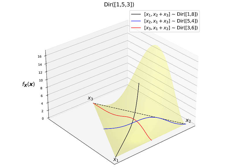

Marginal distributions

Now using the aggregation property, we can find the marginal distributions of Dirichlet distributions when X has more than 2 elements. Let X have a Dirichlet distribution:

We can apply the aggregation property repeatedly on all the elements of X except X₁, and we get:

We can write the previous equation as

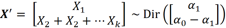
where

More generally, we can write the same equation for each element of X:

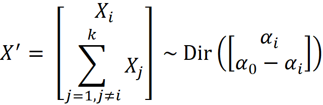
Hence, based on Equation 13, the marginal distribution of each Xᵢ is the following beta distribution:

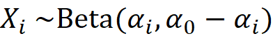
In this article, we reviewed the Dirichlet distribution. We showed that it is the conjugate prior to the multinomial distribution, and due to this important property, it can be used to infer the parameters of the multinomial distribution. We also showed how it can be modeled in Python and how we can visualize its joint PDF. Finally, we saw the connection between the beta and Dirichlet distributions and showed that the Dirichlet distribution is a generalization of the beta distribution to higher dimensions.

I hope that you enjoyed reading this article. Please let me know if you have any questions or suggestions. All the Code Listings in this article are available for download as a Jupyter Notebook from GitHub at:

https://github.com/reza-bagheri/probability_distributions/blob/main/dirichlet_distribution.ipynb