Embrace Randomness for Creating Fast Algorithms

Are you really willing to wait for weeks for 100% certainty if you can already have 99.9% within a minute?

Randomized algorithms are a fascinating area of study in computer science. These algorithms use randomness to solve problems quickly and efficiently, usually outperforming deterministic algorithms.

The catch: randomized algorithms may produce incorrect results with some probability, while their deterministic counterparts never err — given they are implemented correctly. However, the error probability is no big issue since we can systematically control it with careful analysis. We can even bring it down arbitrarily close to zero by repeatedly running the randomized algorithms.

Randomized algorithms give us tradeoffs between speed and correctness, which is a nice addition to the time-memory tradeoffs we usually have.

Since randomized algorithms have numerous applications in various vital fields, such as cryptography or machine learning, we will look at their foundations in this article to get you started for your own use cases. We will use Python for the programming parts, but feel free to follow along with any programming language of your choice.

Motivation

As an introductory example, let us use the problem of checking if the multiplication of two matrices worked.

Given three n×n matrices A, B, and C, check if C = A·B.

I took this example from the great book of Mitzenmacher and Upfal [1]. As in the book, let us assume that the matrices are defined modulo 2, i.e., contain only zeroes and ones with the special feature that 1 + 1 = 0. The rest of the addition and multiplication works just as with real numbers.

Check out the following matrix multiplication modulo 2 as an example:

In the top left corner of the right matrix, we used 1 + 1 = 0.

Let us create some matrices before we check out the algorithms to solve this problem.

import numpy as np

N = 2000

np.random.seed(0)
A = np.random.binomial(n=1, p=0.5, size=(N, N)) # random binary matrix
B = np.random.binomial(n=1, p=0.5, size=(N, N)) # random binary matrix
C = np.mod(A @ B, 2)

C[N // 2, N // 2] = 1 - C[N // 2, N // 2] # change C such that A·B ≠ C

Deterministic Algorithm

The straightforward way to check if C = A · B is the following:

1. Compute C’ = A · B.
2. Check if C = C’.

Easy. The problem with this approach is that step 1 is relatively slow. If you implement the matrix multiplication naively, the run time becomes Θ(n³). If you really take it seriously and use the fastest algorithms, you can lower the exponent to about 2.37188 as of today.

def matrix_multiplication_correct_deterministic(A, B, C):
    return np.all(np.mod(A @ B, 2) == C)

This takes about 45 seconds on my machine, which is quite a lot already. The result is False, as expected.

Note: Asymptotically, this is much better, but keep in mind that very often, we introduce some noticeable overhead in the form of constants that get hidden within the big-Oh notation. This means that using the more advanced algorithms often makes sense when the matrix dimensions reach several hundred or even thousand.

Probabilistic Algorithm

What if I tell you that

1. we can do it in time Θ(n²) with a reasonable success probability
2. with an algorithm much simpler than any advanced matrix multiplication algorithm?

If you don’t believe me, read on. If you do, also read on.

Initial Version

The idea of the algorithm is as follows:

Choose a random binary vector r. If A · (B · r) ≠ C · r, then A·B ≠ C, definitely. Otherwise, maybe A · B = C.

Wow, that’s very easy as well, and the implementation is simple as well.

def matrix_multiplication_correct_probabilistic(A, B, C):
    r = np.random.binomial(n=1, p=0.5, size=N) # random binary vector

    return np.all(np.mod(A @ (B @ r), 2) == np.mod(C @ r, 2))

If you execute this algorithm, you will first notice that it is fast, about 25 milliseconds for me, which is more than 1000 times faster than before. That is because we only do matrix-vector multiplications here — three in total — with a run time of Θ(n²) each.

However, if you execute it a few more times, you will see that in half of the cases, it returns True, and in the other half, False.

Congratulations, you have implemented a coin in a complicated way (so far).

What went wrong?

The way we designed the matrices A, B, and C, we clearly have A · B ≠ C. Still, somehow in about 50% of the cases, we have A · (B · r) = C · r. This is a bad event we do not want since the algorithm outputs the wrong decision.

We must change something about this to make this algorithm useful. But first — and this is usually the most challenging part when designing probabilistic algorithms — we have to upper-bound the error probability.

It turns out that whenever we have A · B ≠ C, the probability for a (uniformly) random binary r obeying A · (B · r) = C · r — this is a bad event when the algorithm fails — is less than 50%. In our special case, with only a single entry in C changed, it is exactly 50%. If we change even more values in C, the algorithm has a lower fail probability.

For the math nerds: The probability is P(fail) = 0.5^rank(A · B - C), so it follows that P(success) = P(A · (B · r) ≠ C · r) = 1 - 0.5^rank(A · B - C) in case of A · B ≠ C.

We will not compute this here, meaning we will sweep the most challenging part under the rug. Be aware of that. The proof is not difficult in this case, yet it takes more time to understand than the actual algorithm, which is often the case.

Furthermore, we have already seen empirically that it fails with a 50% probability. In summary, we have the following:

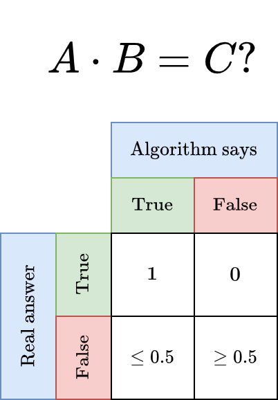
In words: if A · B = C (real answer = True), the probabilistic algorithm will always output the correct answer. Otherwise, it’s a coin flip in the worst case.

Boosting The Success Probability

The good news: we can use a technique called boosting to improve the success probability. This is just a fancy way of saying:

Choose k random binary vectors r. If A · (B · r) ≠ C · r for any of them, then A·B ≠ C, definitely. Otherwise, maybe we have A · B = C.

In code:

def matrix_multiplication_correct_probabilistic_boosted(A, B, C, k):
    for _ in range(k): # many trials
        r = np.random.binomial(n=1, p=0.5, size=N)
        if np.any(np.mod(A @ (B @ r), 2) != np.mod(C @ r, 2)): # early stop, definitely A·B≠C
            return False
    return True

Intuitively, this repetition helps because the algorithm only mistakenly outputs True if it is really unlucky: all randomly chosen vectors r have to obey A · (B · r) = C · r. Each and every one of them. For one, the probability was less than 0.5, so the probability for k independently samples r is less than 0.5ᵏ by the laws of probability.

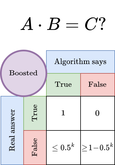
Nice! And what does it cost? Only a factor of k:

The run time of the boosted algorithm is O(k · n²).

Already setting k = 10 gives us an algorithm with a success probability of more than 99.9%, which is often more than enough.

This algorithm still only takes a few milliseconds to execute. Sometimes a bit more than before (at most k = 10 times in our case), but often even the first tested r is enough to output False already, which results in a similar run time of about 25 milliseconds. Cool!

Conclusion

Randomized algorithms are efficient solutions for a variety of problems. However, they do come with the risk of producing incorrect results. Luckily, we can often lower this risk to nearly zero, but never precisely zero. If this is unacceptable in your use case, do not use them.

In any other case, I encourage you to try to develop a probabilistic solution. As seen in the matrix multiplication example, coming up with an idea for a probabilistic algorithm can be extremely simple. Another simple example is checking if two polynomials are equal without resolving all the parenthesis.

The most difficult part about probabilistic algorithms is the mathematics involved in calculating the success probability. If you can do it, you should do it because then you can be sure about how likely your algorithm is to work. With this knowledge, you can even set the parameters of your algorithm to achieve your target success probability, say, 99.9%.

If you do not have the theoretical foundations, check at least empirically if the success probability is large enough. Or ask your friendly mathematician from next door. 😉

Bonus: And what about real-valued matrices? Easy, also just sample a random r, with each component normally distributed around zero. The resulting algorithm has a likelihood to succeed of 100%. Try it out! In this special case, you can have it fast and accurate.

References

[1] Mitzenmacher, M., & Upfal, E. (2017). Probability and computing: Randomization and probabilistic techniques in algorithms and data analysis. Cambridge university press.

I hope that you learned something new, interesting, and valuable today. Thanks for reading!

If you have any questions, write me on LinkedIn!