
Elements of Neural Networks
Activation Functions:
Introduction:
The Internet provides access to a plethora of information today. Whatever we need is just a Google (search) away. However, when we have so much information, the challenge is to segregate between relevant and irrelevant information.
When our brain is fed with a lot of information simultaneously, it tries hard to understand and classify the information into “useful” and “not-so-useful” information. We need a similar mechanism for classifying incoming information as “useful” or “less-useful” in the case of Neural Networks.
This is important in the way a network learns because not all the information is equally useful. Some of it is just noise. This is where activation functions come into the picture. The activation functions help the network use important information and suppress irrelevant data points.
Let us go through these activation functions, learn how they work, and figure out which activation functions fit well into what kind of problem statement.
Brief Overview of Neural Networks:
Before I dive into the details of activation functions, let us quickly go through the concept of neural networks and how they work. A neural network is a very powerful machine learning mechanism which basically mimics how a human brain learns.
The brain receives the stimulus from the outside world, does the processing on the input, and then generates the output. As the task gets complicated, multiple neurons form a complex network, passing information among themselves.
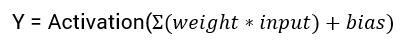
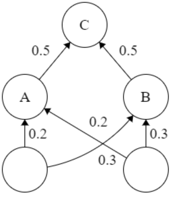
An Artificial Neural Network tries to mimic a similar behavior. The network you see below is a neural network made of interconnected neurons. Each neuron is characterized by its weight, bias, and activation function.
The input is fed to the input layer, the neurons perform a linear transformation on this input using the weights and biases.
x = (weight * input) + bias
Post that, an activation function is applied to the above result.
Finally, the output from the activation function moves to the next hidden layer and the same process is repeated. This forward movement of information is known as the forward propagation.
What if the output generated is far away from the actual value? Using the output from the forward propagation, the error is calculated. Based on this error value, the weights and biases of the neurons are updated. This process is known as back-propagation.
Can we do without an activation function?
We understand that using an activation function introduces an additional step at each layer during the forward propagation. Now the question is — if the activation function increases the complexity so much, can we do without an activation function?
Imagine a neural network without the activation functions. In that case, every neuron will only be performing a linear transformation on the inputs using the weights and biases. Although linear transformations make the neural network simpler, this network would be less powerful and will not be able to learn the complex patterns from the data.
A neural network without an activation function is essentially just a linear regression model.
Thus we use a non-linear transformation to the inputs of the neuron and this non-linearity in the network is introduced by an activation function.
In the next section, we will look at the different types of Activation Functions.
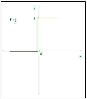
Binary Step Function:
A binary step function is a threshold-based activation function. If the input value is above or below a certain threshold, the neuron is activated and sends exactly the same signal to the next layer.
The problem with a step function is that it does not allow multi-value outputs — for example, it cannot support classifying the inputs into one of several categories.
Mathematically,
f(x) = 1, x >= 0
= 0, x < 0
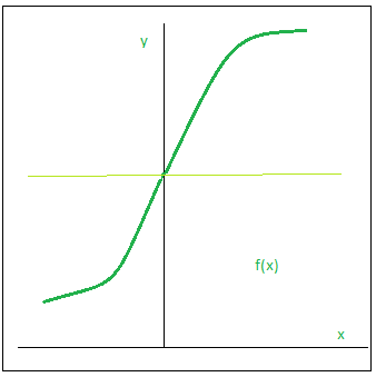
Sigmoid
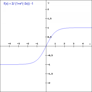
The next activation function that we are going to look at is the Sigmoid function. It is one of the most widely used non-linear activation function. Sigmoid transforms the values between the range 0 and 1.
Here is the mathematical expression for sigmoid- f(x) = 1/(1+e^-x)
Advantages:
- Smooth gradient, preventing “jumps” in output values.
- Output values bound between 0 and 1, normalizing the output of each neuron.
- Clear predictions — For X above 2 or below -2, tends to bring the Y value (the prediction) to the edge of the curve, very close to 1 or 0. This enables clear predictions.
Tanh
The tanh function is very similar to the sigmoid function. The only difference is that it is symmetric around the origin. The range of values in this case is from -1 to 1. Thus the inputs to the next layers will not always be of the same sign.
The tanh function is defined as- tanh(x) = 2sigmoid(2x) — 1
Advantages
- Zero centered — making it easier to model inputs that have strongly negative, neutral, and strongly positive values.
- Otherwise like the Sigmoid function.
ReLU
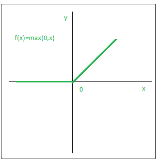
The ReLU function is another non-linear activation function that has gained popularity in the deep learning domain. ReLU stands for Rectified Linear Unit. The neurons will only be deactivated if the output of the linear transformation is less than 0.
The plot below will help you understand this better- f(x) = max(0,x)
Advantages
- Computationally efficient — allows the network to converge very quickly
- Non-linear — although it looks like a linear function, ReLU has a derivative function and allows for backpropagation
Disadvantages
- The Dying ReLU problem — when inputs approach zero, or are negative, the gradient of the function becomes zero, the network cannot perform backpropagation and cannot learn.
Leaky ReLU
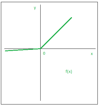
Leaky ReLU function is nothing but an improved version of the ReLU function. As we saw that for the ReLU function, the gradient is 0 for x<0, which would deactivate the neurons in that region.
Leaky ReLU is defined to address this problem. Instead of defining the Relu function as 0 for negative values of x, we define it as an extremely small linear component of x. Here is the mathematical expression-
f(x) = 0.01x , x < 0
= x , x >= 0
Advantages
- Prevents dying ReLU problem — this variation of ReLU has a small positive slope in the negative area, so it does enable backpropagation, even for negative input values
- Otherwise like ReLU
Swish
Swish is a lesser known activation function which was discovered by researchers at Google. Swish is as computationally efficient as ReLU and shows better performance than ReLU on deeper models. The values for swish ranges from negative infinity to infinity. The function is defined as –
f(x) = x*sigmoid(x)
f(x) = x/(1-e^-x)
Softmax:
Unlike binary classification (0 or 1), we need multiple probabilities at the output layer of the neural network. In other words, the number of hidden units in the output layer is equal to the number of classes. For e.g., we want to recognize cats, dogs, and hens from the given dataset. We can classify cats as class 1, dogs as class 2, hens as class 3 and class 0 for none of the above. In such a case, the output layer will have four activation units (4 x 1 matrix). Each activation unit calculates the probability of its respective class and the sum of all elements shall be one.
The softmax function or normalized exponential function can be used to represent a categorical distribution i.e. a probability distribution over ‘K’ different possible outcomes. In simple words, what is the probability that the given picture is of cat or dog or hen or none of these?
Advantages
- Able to handle multiple classes only one class in other activation functions — normalizes the outputs for each class between 0 and 1, and divides by their sum, giving the probability of the input value being in a specific class.
- Useful for output neurons — typically Softmax is used only for the output layer, for neural networks that need to classify inputs into multiple categories.
Learning Rate:
If we wish to understand what learning rates are and why they are there, we must first take a look at the high-level machine learning process for supervised learning scenarios:
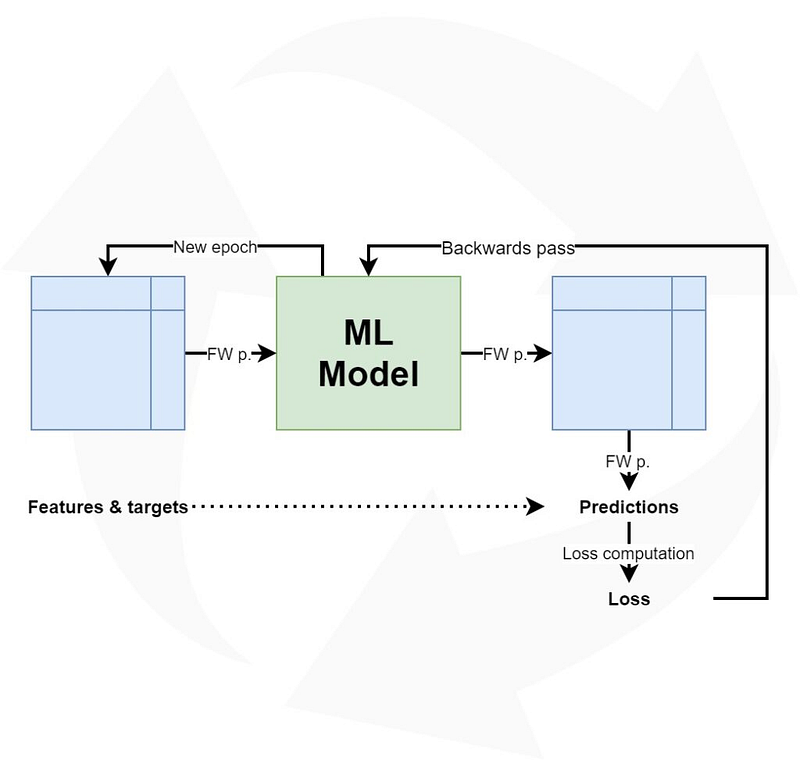
Feeding data forward and computing loss
As you can see, neural networks improve iteratively. This is done by feeding the training data forward, generating a prediction for every sample fed to the model. When comparing the predictions with the actual (known) targets by means of a loss function, it’s possible to determine how well (or, strictly speaking, how bad) the model performs.
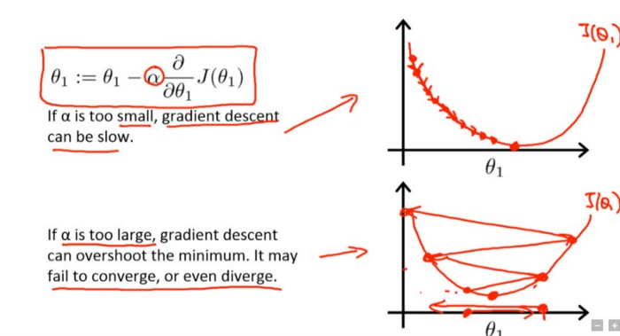
Learning rate is a hyper-parameter that controls how much we are adjusting the weights of our network with respect the loss gradient. The lower the value, the slower we travel along the downward slope. While this might be a good idea (using a low learning rate) in terms of making sure that we do not miss any local minima, it could also mean that we’ll be taking a long time to converge
The following formula shows the relationship:
new_weight = existing_weight — learning_rate * gradient
Dropout:
Deep neural nets with a large number of parameters are very powerful machine learning systems. However, overfitting is a serious problem in such networks. Large networks are also slow to use, making it difficult to deal with overfitting by combining the predictions of many different large neural nets at test time. Dropout is a technique for addressing this problem. The key idea is to randomly drop units (along with their connections) from the neural network during training. This prevents units from co-adapting too much.
Read more here: Dropout: A Simple Way to Prevent Neural Networks from Overfitting
Problem:
When a fully-connected layer has a large number of neurons, co-adaption is more likely to happen. Co-adaptation refers to when multiple neurons in a layer extract the same, or very similar, hidden features from the input data. This can happen when the connection weights for two different neurons are nearly identical.
This poses two different problems to our model:
- Wastage of machine’s resources when computing the same output.
- If many neurons are extracting the same features, it adds more significance to those features for our model. This leads to overfitting if the duplicate extracted features are specific to only the training set.
Batch Normalization:
Training Deep Neural Networks is complicated by the fact that the distribution of each layer’s inputs changes during training, as the parameters of the previous layers change.
This slows down the training by requiring lower learning rates and careful parameter initialization, and makes it notoriously hard to train models with saturating nonlinearities.
We refer to this phenomenon as internal covariate shift, and address the problem by normalizing layer inputs.
Our method draws its strength from making normalization a part of the model architecture and performing the normalization for each training mini-batch.
Batch Normalization allows us to use much higher learning rates and be less careful about initialization.
It also acts as a regularizer, in some cases eliminating the need for Dropout.
Applied to a state-of-the-art image classification model, Batch Normalization achieves the same accuracy with 14 times fewer training steps, and beats the original model by a significant margin.
Read more here: Why Batch Normalization?
Some interactive resources:
- Visualising Activation Functions in Neural Networks
- Tinker With a Neural Network Right in Your Browser.
Gain Access to Expert View — Subscribe to DDI Intel