Efficient Similarity Search & Clustering of Dense Vectors in Neo4j

Scalable Similarity Search of GPT-3 Text Embeddings

by Joshua Yu

Overview of GPT-3 Dense Embeddings

Text embedding is the process of representing text data in a continuous, dense, and meaningful high-dimensional vector space, usually referred to as an embedding space. The goal of text embedding is to map text data into a continuous vector representation that can be used as input to various machine learning algorithms, such as text classification, text generation, and text clustering.

During the embedding process, similar words are represented by similar vectors, and the distance between two vectors represents the similarity between the words they represent. There are already many ways to embed text data, including frequency-based embeddings, such as bag-of-words and term frequency-inverse document frequency (TF-IDF), and dense embeddings, such as word2vec, GloVe, and FastText.

Embeddings generated by GPT-3 are dense embeddings, which are generated using a transformer-based neural network architecture that processes text in a deep and nonlinear way, producing dense vector representations for each token in the input text.

In the 3rd part of my trilogy on Building An Academic Knowledge Graph with OpenAI & Graph Database, I demonstrated a method to use OpenAI embedding API to obtain and store text embeddings of academic paper titles in Neo4j graph database, get embeddings for the search phrase and then use Cosine Similarity to find the most similar titles for that particular search phrase.

Making the Similarity Search More Scalable

In the Academic Paper knowledge Graph, there were only 100 paper titles, doing an one-to-one computation of Cosine Similary between embeddings of the search phrase and title is a trivial task. However, considering a knowledge graph like this can easily grow to tens of millions of titles (as of now, there are already 2.2 millions of papers in the arXiv repository), plus abstract, references and even every paragraph, the above method won’t be scalable at all.

We are used to use index for fast search, then why can’t we create some kind of index of dense vectors to boost search performance too? In fact, there is the solution:

1) using au unsupervised process to cluser embeddings into partitions so that every embedding has the shortest distance to the center of its own cluster, but far awar from those of other clusters.

2) the centers of the cluster (which itself is also a vector) is used to compute the similarity between itself and the vector of the search phrase, and only the most similar center(s) are used to do further similarity search within their partitions.

In order to achieve these functions, there are some mathematical concepts to explain first.

1. k-means Clustering

k-means Clustering is a quite popular algorithm used for partitioning a set of data points into k clusters. You can find a more comprehensive definition of it on wikipedia, but I’ll use a version generated by ChatGPT in plain English as per my instruction:

The k-means algorithm tries to find k points, called centroids, that represent the center of each cluster.

To do this, the algorithm first selects k random data points as the initial centroids. It then assigns each data point to the nearest centroid based on its distance from the centroid. Next, the algorithm calculates the mean of all the data points assigned to each centroid and updates the centroid to this mean. It repeats this process until the centroids no longer change or a maximum number of iterations is reached.

Apparently, how to decide the best k is the tricky part here. Ideally, k should be equal to the number of clusters, which needs to be decided through iterations. This comes to our next key concept, i.e. silhoutte.

2. Silhoutte

Before I explain the meaning of silhoutte, let’s me try to pronounce it correctly first. It was a French word satirically derived from the name of the parsimonious mid-18th-century French finance minister Étienne de Silhouette, whose hobby was the cutting of paper shadow portraits.

I really had no idea why the surname of a politician was named for his hobby, and then selected here, but the only thing to remember is it has a range of [-1, 1], and the higher value means the object is better matched to its own cluster. Again you can find a comprehensive mathematical explanation of it on wikipedia.

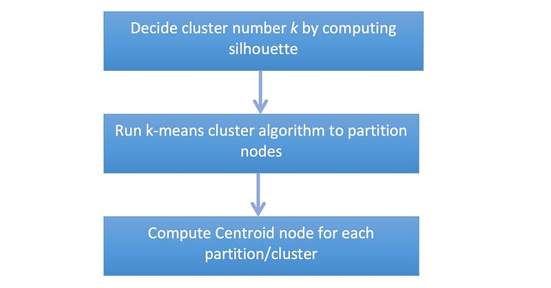
With this little extra knowledge of maths, we can come up with the process of clustering vectors (stored as property in our Academic Paper Knowledge Graph):

Implementing Index for Dense Vectors

1. What We Need

• Neo4j Desktop with Enterprise Graph Database
• Neo4j Graph Data Science 2.3 plugin installed within Neo4j Desktop
• Python 3.9 and Jupyter or MSCode for data visualisation
• The Academic Paper Knowledge Graph

For steps of having Neo4j Desktop and GDS plugin installed, you may refer to the 3rd part of my trilogy on Building An Academic Knowledge Graph with OpenAI & Graph Database.

Alternatively, Neo4j AuraDS, the DaaS version of both Neo4j Graph database and GDS, can be an easier choice if you don’t mind putting down several dollars for running it.

To make this more obvious to verify, I also loaded papers from arXiv using these 3 search phrases:

a. graph neural network: 100 titles

b. computer vision: 50 titles

c. material: 50 titles

2. Find out The Best k

Neo4j Graph Data Science library already comes with the k-means clustering algorithm. Like any other graph algorithms in the library, it has four ways to execute:

i) Stream: run and return results.

ii) Stats: return statistics of execution only.

iii) Mutate: run in memory only.

iv) Write: run and write results to specified property in database.

To find out the best k, I will use a strategy similar to the Elbow Method, i.e. let k start from 2 to the square root of total nodes ( sqrt(200) = 14), and calculate average silhoutte value, and choose the k where there is the Elbow. Cypher statements are given below:

//  1) k-mean : graph projection
CALL gds.graph.project(
    'title-graph',
    {
      Title: {
        properties: 'embedding'
      }
    },
    'HAS_TITLE'
);

//   2) k-mean : decide the best k

WITH range(2,14) AS kcol
UNWIND kcol AS k
CALL gds.beta.kmeans.stream(
    'title-graph',
    {
        nodeProperty: 'embedding',
        computeSilhouette: true,
        k: k
    }
) YIELD nodeId, communityId, silhouette
WITH k, avg(silhouette) AS avgSilhouette
RETURN k, avgSilhouette;

The chart below shows how average silhoutte value changes together with different k:

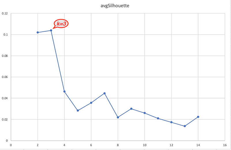
When k = 3, the average silhoutte value is the maximum (still remember its definition?) which indicates 3 is the best value for k.

3. Partition Nodes into k Clusters

Now we have found the best k, the next step is to actually run the algorithm to partition Title nodes, and save cluster number as a new property km-1536-cluster of the Title nodes.

//   3) k-mean : cluster nodes using the best k

CALL gds.beta.kmeans.write(
    'title-graph',
    {
        nodeProperty: 'embedding',
        writeProperty: 'km-1536-cluster',
        k: 3
    }
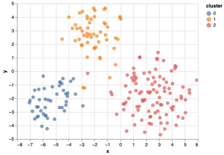
) YIELD nodePropertiesWritten;

Plotting to a 2-dimension space, it clearly shows 3 clusters that are seperated properly:

4. Generate Centroid Nodes

Centroid node is the center of each cluster. I simply use average of all vectors of the cluster as its vector. In Neo4j, vectors are stored as a List of Float, and because vectors are generated by OpenAI Embedding API, it has a dimension of 1536.

//    4) compute centroid nodes

:param embedding_size=>1536;

MATCH (u:Title) 
WITH u.`km-1536-cluster` AS cluster, u, range(0, $embedding_size) AS ii 
UNWIND ii AS i
WITH cluster, i, avg(u.`embedding`[i]) AS avgVal
ORDER BY cluster, i
WITH cluster, collect(avgVal) AS avgEmbeddings
MERGE (cl:Centroid{method: 'text-embedding-ada-002', dimension: $embedding_size, cluster: cluster})
    SET cl.embedding = avgEmbeddings
RETURN cl;

5. Validate the Results

The steps above are all we need! Now let’s visualize the results. Here I used Neo4j Python driver to connect to the database and run a query to get embeddings of all Title & Centroid nodes, together with the cluster Id of Titles. The visualization package is Altair, as I found it is quite powerful and easy to use .

from neo4j import GraphDatabase

# Connect to Neo4j
uri = "neo4j://localhost:7687"
driver = GraphDatabase.driver(uri, auth=("neo4j", "***PASSWORD***"), database="academic")

# Show results in DataFrame
with driver.session() as session:
    result = session.run("""
              MATCH (t:Title) RETURN 'Title' AS label, t.text AS text, toString(t.`km-1536-cluster`) AS cluster, t.embedding AS embedding 
              UNION ALL 
              MATCH (c:Centroid) WHERE c.method = 'text-embedding-ada-002' RETURN 'Centroid' AS label, toString(c.cluster) AS text, c.cluster AS cluster, c.embedding AS embedding;
    """, {})
    
    df1 = pd.DataFrame([dict(record) for record in result])
    print(df1)

from sklearn.manifold import TSNE
import numpy as np
import matplotlib.pyplot as plt
import altair as alt

# Load group labels for each data point
group1 = df1.cluster
group2 = df1.label
group3 = df1.text

# Set up t-SNE object and fit data
tsne = TSNE(n_components=2, perplexity=30, learning_rate=400)
X_tsne = tsne.fit_transform(list(df1.embedding))

df = pd.DataFrame(data = {
    "text": group3,
    "label": group2,
    "x": [value[0] for value in X_tsne],
    "y": [value[1] for value in X_tsne]
})

alt.data_transformers.disable_max_rows()

alt.Chart(df).mark_circle(size=60).encode(
    x='x',
    y='y',
    color='label',
    tooltip=['text']
).interactive()

And the plotting:

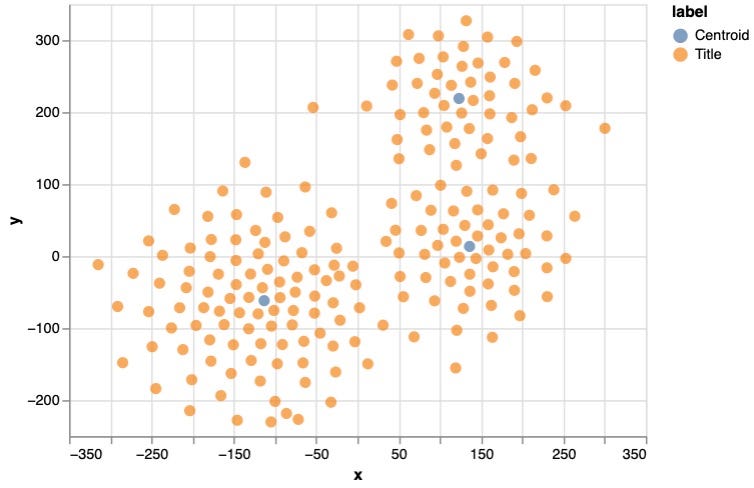
Further Discussion

With Centroid Nodes created and used as some kind of Index, the similarity seach of vectors can firstly be done between seach phrase and centroids, and then within the matched cluster(s). This can largely reduce the computation workload. A benchmark test of search over 1 million vectors of 1536 dimensions is shared below (using Cosine Similarity), using single thread:

> full scan of all vectors : over 190 seconds

> match 1000 centroids and return top 50 titles in a cluster: < 300ms

Because k-means algorithm is computationally difficult (NP-Hard), for larger graph, some strategy like sampling could be used to approximate the results while maintaining reasonable accuracy.

There are similar solutions for vector search, e.g. Facebook’s FAISS, however with the support from database query language and Graph Data Science library, I’ve demonstrated a native solution which runs perfectly well on the knowledge graph.