Summary

The website content discusses the evolution of neural network scaling, highlighting the transition from VGG16 to Efficient Nets, which utilize a compound scaling method to optimize performance and computational efficiency.

Abstract

The text outlines the historical challenges in scaling neural networks, particularly before the invention of Batchnorm in 2014, which hindered the training of complex models like VGG16. It explains that scaling in depth, width, and resolution is crucial for network performance, as it allows for the extraction of features at different scales and resolutions, akin to varying the resolution of a microscope. The ancient VGG16 architecture is described as linearly scaled and less effective for complex tasks compared to the state-of-the-art Efficient Nets developed by Google. Efficient Nets employ a compound scaling method that uses a coefficient φ to uniformly scale network depth, width, and resolution, optimizing resource allocation and improving accuracy while maintaining low computational complexity. The method constrains the scaling coefficients α, β, and γ such that the total FLOPS increase by approximately 2^φ, ensuring efficient use of computational resources. The performance gains from compound scaling are demonstrated through class activation maps and top-1% accuracy vs. FLOPS graphs, showing Efficient Net's superiority over other models. The text also mentions the model-agnostic nature of compound scaling and notes that Efficient Net B6 wide is a top performer in the ImageNet challenge.

Opinions

The author suggests that the invention of Batchnorm was a pivotal moment in the development of neural networks, implying that it was a significant barrier to progress before 2014.
The author expresses that simply adding layers of the same size and resolution is not optimal due to the increased number of parameters and memory requirements, as well as the need to capture hidden patterns at different scales.
The text conveys a clear preference for Efficient Nets over older architectures like VGG16, emphasizing their effectiveness in complex tasks and their state-of-the-art status.
The author seems to appreciate the balance struck by compound scaling between model complexity and computational efficiency, noting its principled approach to resource allocation.
The author implies that the compound scaling method is universally applicable, as it is model-agnostic and can be used to improve various types of ConvNets.
There is an acknowledgment of the community's benchmarking practices, as the author points out that new models are evaluated against the ImageNet dataset, reinforcing its role as a standard for comparing model performance.

Efficient Nets: Scaling of Conv networks

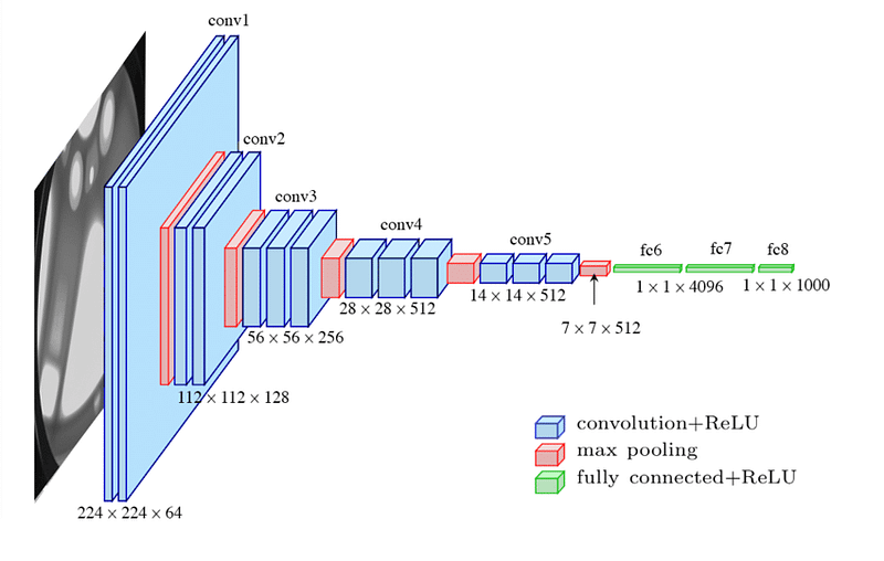
Because of scaling, neural networks took so many years to come forward despite all its maths already being present since the 90s. Back then, we didn’t understand properly how to make a neural network work for complex tasks. Since Batchnorm() was not invented until 2014, researchers struggled to train VGG16. Basically, we didn’t understand how to scale the networks to perform complex tasks. If you’ll look at the VGG16 architecture below image, you’ll observe scaling happening at three different levels: Depth, width, and resolution.

Depth scaling is the number of layers in a given network. Width scaling is the size of each Conv layer {112x112 or 56x56} and resolution is the depth of each Conv layer {112x112x128 (resolution =128)}. But, why do we need scaling? Why can’t we just add the same size and resolution layers and make predictions using that? There are two reasons why we don’t do that, firstly, using the same size layers will cause a huge jump in the number of parameters (more parameters means more memory requirements) and secondly, we want features to be read at different scales so that we can find more hidden patterns in the data stream(imagine the resolution of Conv layers as the resolution of a microscope). You can choose these numbers (scaling parameters) but the model’s performance won’t be optimized. Correct scaling is the key to a model’s success.

As of now, VGG16 is considered ancient and its scaling is very linear thus it fails in complex tasks. In recent times, Efficient Net has gained huge popularity because of its dynamic scaling. Efficient Net is considered to be the state of the art developed by google. It combines a compound scaling methodology to achieve a considerable improvement in accuracy and low computational complexity.

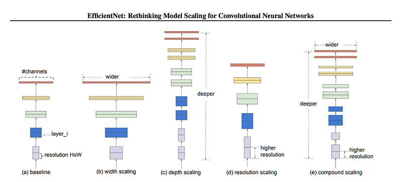
Compound scaling: The compound scaling method uses a compound coefficient φ to uniformly scale network width, depth, and resolution in a principled way:

depth: d = α ^φ

width: w = β ^φ

resolution: r = γ^ φ

s.t. α · β^ 2 · γ^ 2 ≈ 2

α ≥ 1, β ≥ 1, γ ≥ 1

Here α, β, γ are constants that can be determined by a small grid search. Intuitively, φ is a user-specified coefficient that controls how many more resources are available for model scaling, while α, β, γ specify how to assign these extra resources to network width, depth, and resolution, respectively. Notably, the FLOPS of a regular convolution op is proportional to d, w^2, r^ 2, i.e., doubling network depth will double FLOPS, but doubling network width or resolution will increase FLOPS by four times. Since convolution ops usually dominate the computation cost in ConvNets, scaling a ConvNet with equation 3 will approximately increase total FLOPS by (α · β 2 · γ 2) ^φ. In this paper, we constraint α · β ^2 · γ^ 2 ≈ 2 such that for any new φ, the total FLOPS will approximately increase by 2^φ.

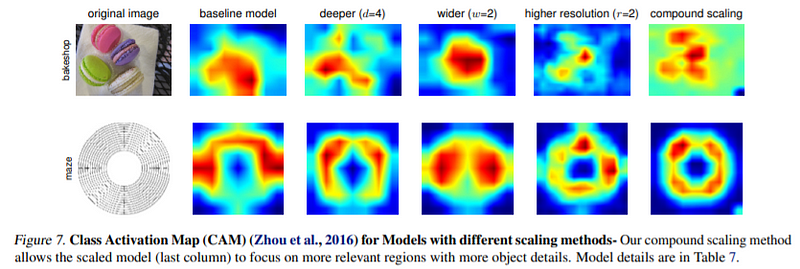
All we discussed above sounds good in theory, but how does it translate to actual performance. In DL, performance is often looked at through the value of loss or some other metric. A better way to understand networks' performance is to look at the class activation map, which basically tells us what a network finds salient or essential in a given image. You can see the improvement in performance due to compound scaling.

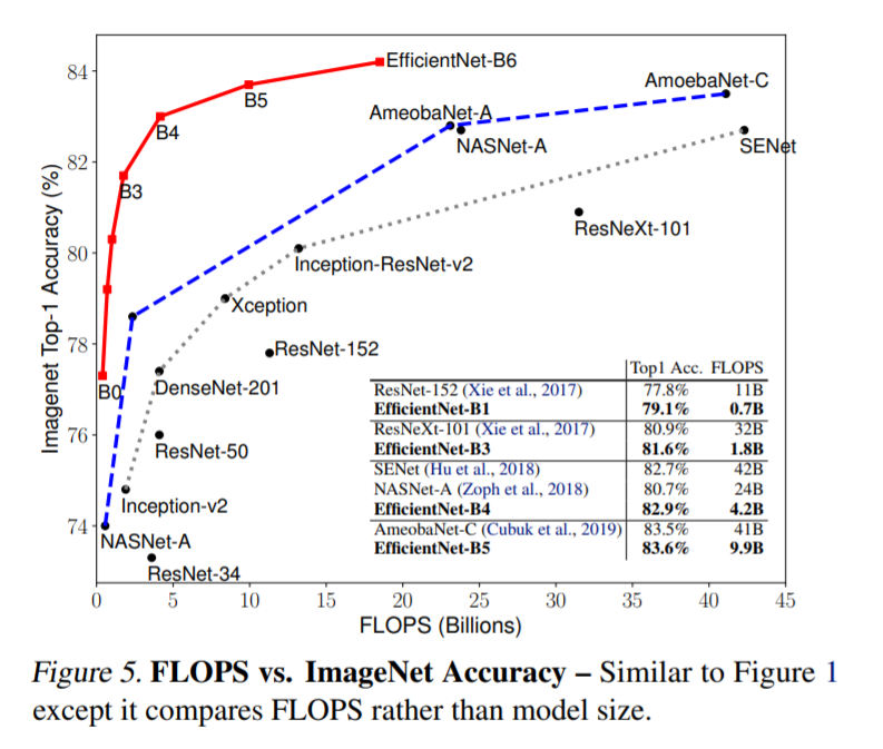
For the more nerdy people, here’s the graph of top-1% accuracy vs FLOPS (number of operations) for different state-of-the-art models. We can see that efficient Net achieves much higher performance for fewer parameters or FLOPS.

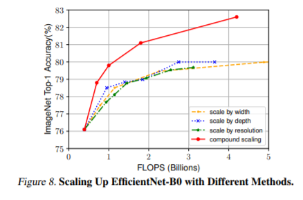
And also, in the graph for the effect of different scaling, we see similar results, huge improvement through compound scaling over traditional scaling. The idea behind Efficient Net is straightforward but a compelling one. Another good thing about Compound scaling is that it’s model agnostic (model-independent). As of writing this blog, Efficient Net B6 wide is the best model in the world for the Imagenet challenge (All the new models are benchmarked on this dataset only).

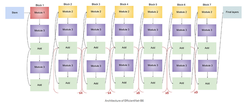
And if you are wondering what’s with the different Efficient net B1, B2…B6, architecture, they just have more layers than their previous version, thus a better ability to extract more deep features. The earlier versions of Efficient Net have similar architecture and lesser connections compared to B6 and B7. Going into the architecture detail is beyond the scope of this particular blog.

Join Medium with my referral link - Vishal Rajput

As a Medium member, a portion of your membership fee goes to writers you read, and you get full access to every story…

vishal-ai.medium.com

Thanks for giving your time, and if you think that this blog added something to your knowledge base, please consider following the AI guys Blog, and if you are interested to become a writer at AI Guys you can follow this link.