Efficient Distribution Modeling with Planar Normalizing Flows: A Deep Learning Approach

Abstract

Context: Normalizing flows utilize deep learning to transform simple distributions into complex ones, facilitating efficient sampling and precise probability density evaluation, which is crucial for generative models and statistical inference. Problem: Traditional models need help with direct complex distribution modeling and efficient likelihood computation, especially in high-dimensional spaces. Approach: We implement planar flows to transform a base distribution, focusing on efficient computation of the log determinant of the Jacobian, which is essential for model training and evaluation. Results: The model learns to replicate a synthetic dataset's distribution, demonstrating normalizing flows' capacity to model complex distributions effectively. Computational challenges related to tensor operations are addressed, showcasing the model's adaptability. Conclusions: Normalizing flows, particularly planar flows, offer a powerful method for deep learning-based distribution modeling, balancing expressiveness with computational efficiency. Future efforts will focus on optimizing these models further and expanding their applications.

Keywords: Normalizing Flows; Deep Learning; Generative Models; Probability Distribution Modeling; Planar Flow Implementation.

Introduction

Normalizing flows represent a powerful and flexible class of models within the domain of deep learning designed for modeling complex probability distributions. They operate under a relatively straightforward yet profound concept: transforming a simple, well-understood base distribution (such as a Gaussian or uniform distribution) into a more complex distribution that can represent the intricate patterns in real-world data. This transformation is achieved through a sequence of invertible and differentiable mappings, hence the term "flow." The elegance of normalizing flows lies in their ability to perform two crucial tasks in probabilistic modeling: sampling from the distribution and evaluating the probability density of given samples. This essay delves into the mechanisms of normalizing flows, their significance, and their applications, highlighting their unique position in the landscape of generative modeling.

In the flow of complexity, simplicity finds its strength.

The Mechanism of Normalizing Flows

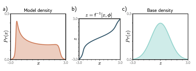
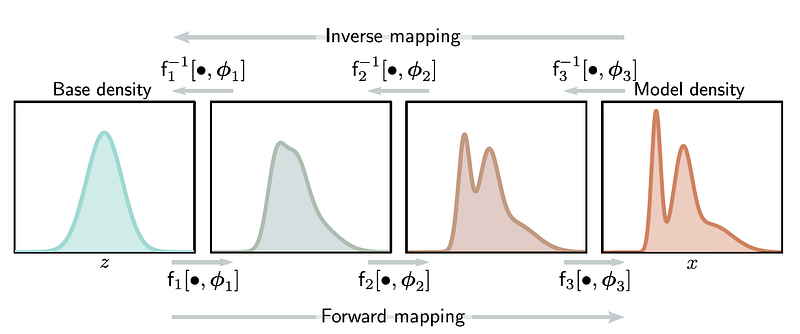
At the heart of normalizing flows is transforming a simple distribution into a more complex one. This is achieved by applying a sequence of invertible functions, where each function is designed to be easily invertible, and its Jacobian determinant — necessary for probability density calculations — can be efficiently computed. The initial simple distribution, often called the base or prior distribution, acts as a starting point, progressively shaping into the target distribution that captures the complexities of the data being modeled.

The transformation process is guided by the principles of change of variables in probability. For a given invertible function, the density of the transformed variable can be calculated if one knows the density of the original variable and the determinant of the function's Jacobian. This principle ensures that as the data undergoes transformations, its probability density can be accurately tracked and updated, allowing sampling and probability evaluation.

Importance and Applications

The dual capability of sampling and probability density evaluation makes normalizing flows exceptionally valuable for various machine learning and data science applications. Generative modeling is one of the most prominent applications, which aims to model and sample from complex data distributions. Normalizing flows enable the generation of high-quality, diverse samples that closely resemble the actual data distribution, applicable in fields such as image and speech synthesis, drug discovery, and anomaly detection.

Furthermore, normalizing flows are used in variational inference, providing a flexible and expressive family of distributions for approximating posterior distributions in Bayesian modeling. This flexibility allows for more accurate inference in complex probabilistic models, enhancing the performance of models across tasks such as predictive modeling, unsupervised learning, and reinforcement learning.

Mathematics Foundations

To clarify the mathematics underlying normalizing flows and specifically the computation involved in the log determinant of the Jacobian, let's break down the relevant equations separately from the explanatory text. This approach will help us focus on the theoretical foundations that guide the implementation of normalizing flows.

Base Concepts

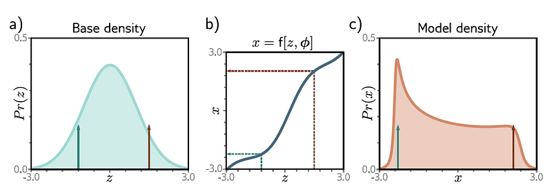
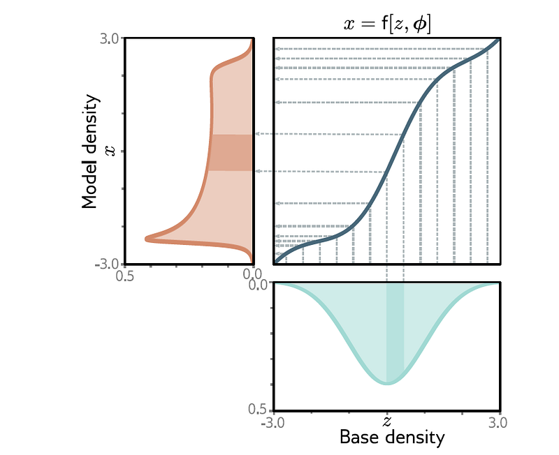
Normalizing flows transform a simple distribution )pz​(z) into a more complex distribution px​(x) using an invertible and differentiable function f. The transformation follows the change of variables formula:

X is a sample from the complex distribution, and z is from the simple base distribution.

Probability Density Function Transformation

The probability density function (PDF) of x can be derived from the PDF of z using the change of variables formula, which includes the determinant of the Jacobian of the transformation f:

Log Determinant of the Jacobian

For efficiency and numerical stability, normalizing flows often work with the logarithm of the determinant of the Jacobian matrix. The Jacobian matrix Jf​(z) for the transformation f is defined as:

Its log determinant is given by:

Planar Flow-Specific Equations

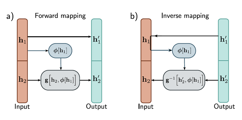
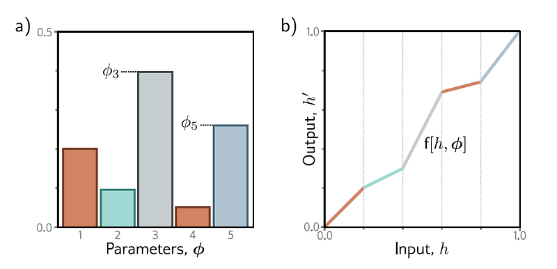
In the context of a planar flow, which is a specific type of normalizing flow, the transformation f is often defined as:

Where:

• z is the input vector.
• u is a learnable parameter vector (akin to self.scale in the implementation).
• w is another learnable parameter vector (akin to self.weight).
• b is a learnable bias parameter (akin to self.bias).
• ℎh is a nonlinear activation function, such as tanh⁡tanh.

The log determinant of the Jacobian for this transformation, taking into account the properties of ℎh, can be computed as:

Where:

• I is the identity matrix.
• ψ is the derivative of the activation function ℎh concerning its input, specifically:

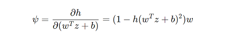
This derivative ψ represents how input z changes affect the activation function's output, modulated by the parameters w and b.

The key to implementing normalizing flows, including planar flows, is efficiently computing these transformations and their log determinants, allowing forward sampling and evaluating log probabilities.

Challenges and Future Directions

Despite their advantages, normalizing flows also face challenges, primarily related to the computational cost and complexity of designing and training deep invertible networks. The requirement for invertibility and efficient computation of the Jacobian determinant often imposes constraints on the architecture of the network, potentially limiting the expressiveness of the model. Moreover, training deep normalizing flows can be resource-intensive, requiring a careful balance between model complexity and computational feasibility.

Ongoing research in normalizing flows aims to address these challenges by developing more efficient and expressive flow architectures, optimizing training algorithms, and exploring new applications. Advances such as continuous normalizing flows, which leverage differential equations to model the transformation process, and autoregressive flows, which increase model expressiveness, highlight the dynamic and evolving nature of research in this area.

Code

Creating a complete example with normalizing flows involves several steps: generating a synthetic dataset, defining the normalizing flow model, training the model on the dataset, evaluating it with appropriate metrics, and visualizing the results. This tutorial will guide you through these steps using Python.

Step 1: Setting up the Environment

Ensure you have the necessary libraries installed. For this example, we'll need PyTorch, a popular deep-learning library that supports normalizing flows, and Matplotlib for visualization.

pip install torch matplotlib

Step 2: Generating a Synthetic Dataset

Let's start with a simple 2D dataset that forms a complex pattern, which our normalizing flow will learn to model.

import numpy as np
import matplotlib.pyplot as plt

def generate_synthetic_data(n_samples=1000):
    x2 = np.random.uniform(-3, 3, n_samples)
    x1 = np.sin(x2) + np.random.normal(0, 0.1, n_samples)
    return np.vstack((x1, x2)).T

# Generate and plot the synthetic dataset
data = generate_synthetic_data()
plt.scatter(data[:, 0], data[:, 1], alpha=0.5)
plt.title('Synthetic Dataset')
plt.xlabel('X1')
plt.ylabel('X2')
plt.show()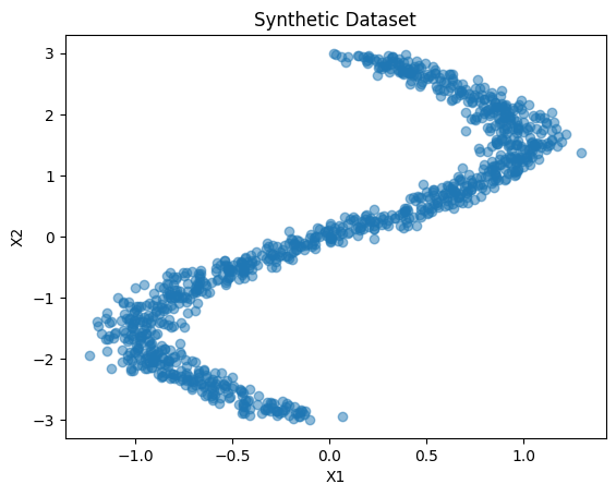

Step 3: Defining the Normalizing Flow Model

We will use a simple planar flow model for demonstration. More complex models like RealNVP or Glow could be used for better performance.

class PlanarFlow(nn.Module):
    def __init__(self, dim):
        super(PlanarFlow, self).__init__()
        self.weight = nn.Parameter(torch.randn(1, dim))  # Adjusted for broadcasting
        self.bias = nn.Parameter(torch.randn(1))
        self.scale = nn.Parameter(torch.randn(1, dim))   # Adjusted for broadcasting

    def forward(self, z):
        # Ensure bias broadcasting works by explicitly matching dimensions
        linear_transformation = torch.matmul(z, self.weight.t()) + self.bias  # Adjust for correct shape
        
        # Activation function
        activation = torch.tanh(linear_transformation)
        
        # Apply scale; ensuring scale is broadcast correctly
        return z + activation * self.scale  # Element-wise multiplication with broadcasting

    def log_det_jacobian(self, z):
        # Calculate the derivative of the activation function
        tanh_z = torch.tanh(torch.matmul(z, self.weight.t()) + self.bias)
        psi = (1 - tanh_z ** 2) @ self.weight  # Derivative of tanh, shape should be compatible with z
        
        # Correct calculation of 'a' for determinant calculation
        # Since direct multiplication is not valid, consider the operation intended by 'a'
        # If 'a' intends to represent a specific transformation, adjust the calculation to fit that purpose.
        
        # For simplicity, assuming 'a' is not directly used but rather demonstrating a concept:
        # Calculate the log determinant considering the derivative 'psi' and the parameter 'scale'
        # Note: This step needs clarification on the intended mathematical operation.
        
        # Assuming a simplified approach where we directly use 'psi' for determinant calculation:
        log_det_jacobian = torch.log(torch.abs(1 + psi @ self.scale.t()))
        
        return log_det_jacobian.squeeze()  # Ensure it returns the correct dimension

Step 4: Training the Model

We'll train the model to learn the distribution of our synthetic dataset.

# Convert data to PyTorch tensor
data_tensor = torch.tensor(data, dtype=torch.float32)

# Model and optimizer
dim = data.shape[1]
flow = PlanarFlow(dim=dim)
optimizer = optim.Adam(flow.parameters(), lr=0.01)

# Training loop
n_epochs = 1000
for epoch in range(n_epochs):
    optimizer.zero_grad()
    z = data_tensor
    transformed_z = flow(z)
    log_det_jacobian = flow.log_det_jacobian(z)
    # Assuming a Gaussian base distribution, compute log-likelihood
    log_likelihood = -0.5 * torch.sum(transformed_z**2, dim=1) + log_det_jacobian
    loss = -torch.mean(log_likelihood)
    loss.backward()
    optimizer.step()

    if epoch % 100 == 0:
        print(f'Epoch {epoch}, Loss: {loss.item()}')

Epoch 0, Loss: 3.198061943054199
Epoch 100, Loss: 0.8239462971687317
Epoch 200, Loss: 0.6688211560249329
Epoch 300, Loss: 0.6594265699386597
Epoch 400, Loss: 0.6583933234214783
Epoch 500, Loss: 0.6575285196304321
Epoch 600, Loss: 0.6563035249710083
Epoch 700, Loss: 0.6545523405075073
Epoch 800, Loss: 0.6520830392837524
Epoch 900, Loss: 0.6487575173377991

Step 5: Evaluating the Model

We'll generate new samples to evaluate the model and compare them visually to the original dataset.

# Sample from base distribution and transform
z_base = torch.randn(1000, dim)
sampled_data = flow(z_base).detach().numpy()

plt.scatter(sampled_data[:, 0], sampled_data[:, 1], alpha=0.5)
plt.title('Samples from Learned Distribution')
plt.xlabel('X1')
plt.ylabel('X2')
plt.show()

Interpretation of Results

By comparing the original dataset and the samples from the learned distribution, we can evaluate how well the normalizing flow has captured the complexity of the data. Ideally, the samples should resemble the structure of the synthetic dataset, indicating that the flow has successfully learned the underlying distribution.

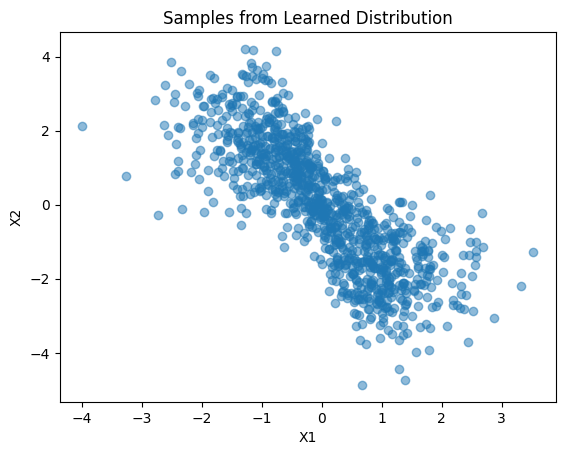
The simplicity of the planar flow model might limit its ability to capture very complex distributions. For more intricate patterns, consider using more advanced normalizing flow architectures.

This tutorial provides a basic framework for implementing and experimenting with normalizing flows. By adjusting the model architecture, training regimen, and dataset, you can explore the vast potential of normalizing flows for modeling complex distributions.

Conclusion

Normalizing flows represents a significant advancement in modeling complex probability distributions through deep learning. By leveraging the power of deep networks to transform simple distributions into intricate real-world data models, normalizing flows provides a versatile tool for sampling and probability density evaluation. Despite facing challenges related to computational efficiency and model design, the ongoing research and development in this field continue to expand its potential applications, making normalizing flows a cornerstone of modern probabilistic modeling and generative deep learning.

In Plain English 🚀

Thank you for being a part of the In Plain English community! Before you go:

• Be sure to clap and follow the writer ️👏️️
• Follow us: X | LinkedIn | YouTube | Discord | Newsletter
• Visit our other platforms: Stackademic | CoFeed | Venture | Cubed
• More content at PlainEnglish.io