
EDA and Feature Engg Series: Handling Missing Values
Exploratory Data Analysis and Feature Engineering Series: Handling missing values & different imputation approaches in practical use case considerations
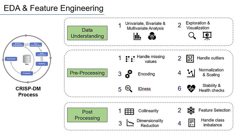
The CRISP-DM methodology in any Data Science program involves key stages around “Data Understanding” and “Data Preparation” phases. We spend majority of our time and effort during these stages.
I will take this opportunity to provide a holistic approach of techniques that we use during these phases in business use cases.
- Data Understanding: Typically involves univariate, bivariate and multivariate analysis, data exploration and data visualization. You may please refer to my previous stories around Data Visualization.
- Pre-Processing: Multiple strategies that can be covered as part of these are as follows: Handling missing values, Handling outliers, Encoding techniques, Normalization and Scaling approaches, Handling IDness, Handling Stability and Drift factors and performing health checks. It depends on our business goal, dataset, scope and context of the use case to see what is relevant and how to approach each of these strategies. At the same time, we must keep in mind about the methods to be followed.
- Post-Processing: This can cover collinearity, feature selection, dimensionality reduction, handling class imbalance and many other aspects.
As part of the series, the focus here is on handling missing values.
Strategy:
- First of all it is important to understand what type the missing values fall into (MCAR or MAR or NMAR/MNAR). This will give us a good idea.
- Secondly, we can plan for strategy for imputation:
a) Ensure to preserve the relations within the dataset
b) Ensure to preserve the uncertainty about these relations
c) Ensure to account for the process that created the missing data
It will help us guide in a step-by-step manner and also result in valid statistical inferences.
3. We will look at most possible methods that are available to handle missingness.
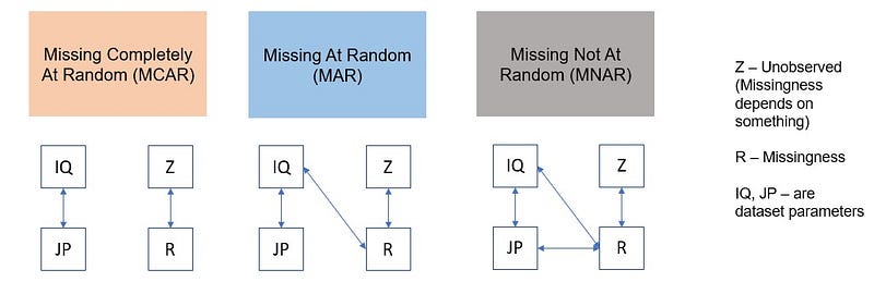
Different Types of missing values:
Some of the examples can be attributed as follows:
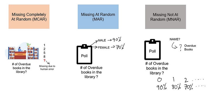
MCAR: For Example, suppose in a library there are some overdue books. Some values of overdue books in the computer system are missing. The reason might be a human error like the librarian forgot to type in the values. So, the missing values of overdue books are not related to any other variable/data in the system. It should not be assumed as it’s a rare case. The advantage of such data is that the statistical analysis remains unbiased. In this case, there is no relationship between the missing data and any other values observed or unobserved (the data which is not recorded) within the given dataset. That is, missing values are completely independent of other data. There is no pattern. In the case of MCAR, the data could be missing due to human error, some system/equipment failure, loss of sample, or some unsatisfactory technicalities while recording the values.
MAR: Missing at random (MAR) means that the reason for missing values can be explained by variables on which you have complete information as there is some relationship between the missing data and other values/data. In this case, the data is not missing for all the observations. It is missing only within sub-samples of the data and there is some pattern in the missing values. For example, if we check the survey data, we may find that all the people have answered their ‘Gender’ but ‘Age’ values are mostly missing for people who have answered their ‘Gender’ as ‘female’. (The reason being most of the females don’t want to reveal their age — could be, just an assumption!!)
MNAR: Missing values depend on the unobserved data. If there is some structure/pattern in missing data and other observed data can not explain it, then it is Missing Not At Random (MNAR). If the missing data does not fall under the MCAR or MAR then it can be categorized as MNAR. It can happen due to the reluctance of people in providing the required information. A specific group of people may not answer some questions in a survey. For example, suppose the name and the number of overdue books are asked in the poll for a library. So most of the people having no overdue books are likely to answer the poll. People having more overdue books are less likely to answer the poll. So in this case, the missing value of the number of overdue books depends on the people who have more books overdue. Another example, people having less income may refuse to share that information in a survey since they may not feel comfortable to reveal the same. In the case of MNAR as well the statistical analysis might result in bias.

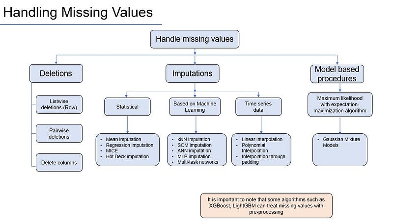
We may or may not use all imputation techniques in most of the practical use cases, however, we should understand the concepts around these so that we can take scientific decision making approach while determining which one to use. There is no thumb rule and it depends on nature of data, business problem and context that we are dealing with and so on..
We can look at 3 broad categories.
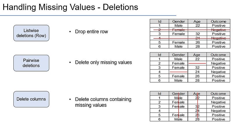
a) Deletions
b) Imputations
c) Model based procedures
I am not going to cover everything here, however few methods will be attempted. Please go through the GitHub here for code example in python.
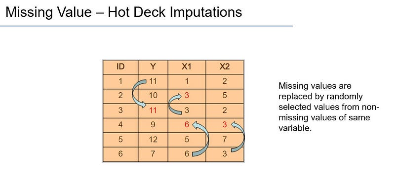
Hot Deck Imputations:
The “Hot Deck Imputation” method is a case with missing value receives valid value from a case randomly chosen from those cases which are maximally similar to the missing one, based on some background variables specified by the user (these variables are also called “deck variables”). The pool of donor cases is called “deck”.
In the most basic scenario — no background characteristics — you might declare the belonging to the same n-cases dataset to be that and only “background variable”; then the imputation will be just random selection from n-m valid cases to be donors for the m cases with missing values. Random substitution is at the core of hot-deck.
In the example illustrated below: The Y variable has a missingness for ID=3, which is replaced by Y value for ID=1, i.e. 11. Similarly, values are replaced randomly from non-missing values of the same variable/feature.
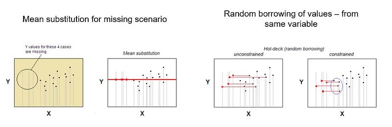
Hot-deck imputation is old still popular because it is both simple in idea and, at the same time, suitable for situations where such methods of processing missing values as listwise deletion or mean/median substitution will not do because missing values are allocated in the data not chaotically — not according to MCAR pattern (Missing Completely At Random). Hot-deck is reasonably suited for MAR pattern (for MNAR, multiple-imputation is the only decent solution). Hot-deck, being random borrowing, does not bias marginal distribution. It, however, potentially affects correlations and biases regressional parameters; this effect, however, could be minimized with more complex/sophisticated versions of hot-deck procedure.
MICE Method:
MICE stands for Multivariate Imputation By Chained Equations algorithm, a technique by which we can effortlessly impute missing values in a dataset by looking at data from other columns and trying to estimate the best prediction for each missing value.
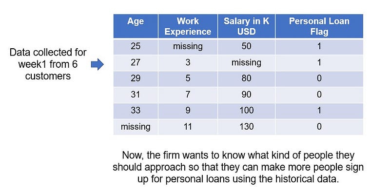
Context: Let’s take an example for a Banking and Financial Services (BFS) major. The sales representative from the leading BFS firm in the world approaches customers to take personal loans.
First step would be to impute the missing values in the data sales rep from the firm collected. Let’s say, the sales rep knows the true values for those missing values, but just wants to see how he can find out if these are missing. So, we will fill in the true values that the sales rep knows.
We will keep this data aside for future reference to cross verify our model if it is good or not.

Remove the “Personal Loan” column as it is the target column, we will not need this column for imputation. We will just impute the 3 feature columns age, experience and salary.
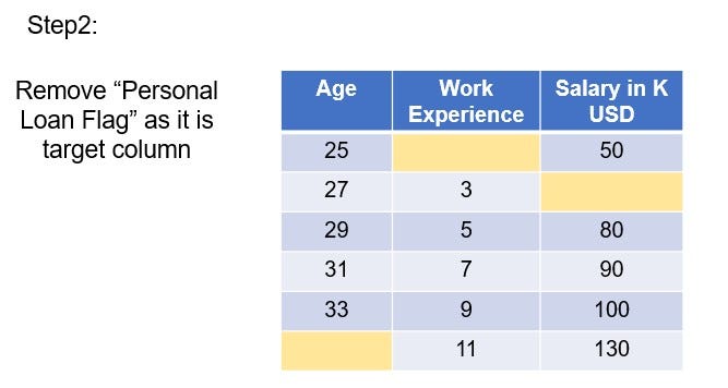
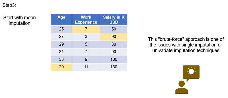
Just by observing the results, we see that a 25 year old has 7 years of IT work experience which is not possible and that too a 7 years experience person earning 50K is totally misleading. And similarly a 29 year old cannot have 11 years of experience. So, we can see that mean imputation is not working as expected. So, this “brute-force” approach is one of the issues with single imputation or univariate imputation techniques.
Multivariate technique solves this issue by factoring in other variables in the data to make better predictions of the missing values. Which means, to find the missing value in age column, we try to run a regression model on the 3 features with experience and salary as features and age as target. Similarly we will try to get the missing values from experience and salary features as well.
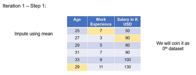
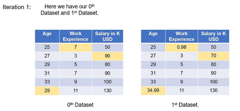
Impute all missing values using mean imputation with the mean of their respective columns.
We will call this as our “0th” dataset
We will be imputing the columns from left to right.
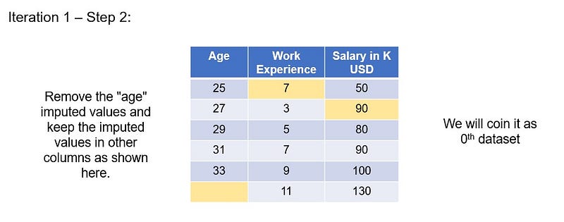
Remove the “age” imputed values and keep the imputed values in other columns as shown here.
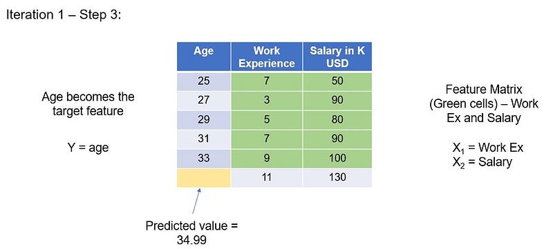
The remaining features and rows(top 5 rows of experience and salary) become the feature matrix(purple cells), “age” becomes the target variable(yellow cells). We will run the linear regression model on the fully filled rows with X= experience and salary and Y=age. To estimate the missing age, we will use the missing value row (white cells) as the test data.
So, top 5 rows will be training data and the last row that has missing age will be test data. We will use (experience = 11 and salary = 130) to predict corresponding “age” value.
When we did this, we found that our model predicted the age as 34.99.
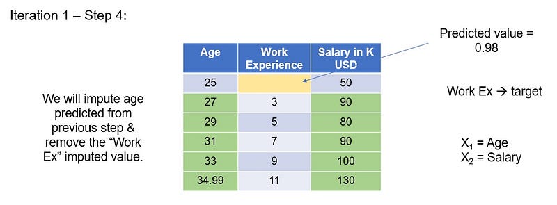
Update the predicted age value in the missing cell in “age” column. Now, remove “experience” imputed value. The remaining features and rows becomes the feature matrix(purple cells) and “experience” becomes the target variable(yellow cells). We will run the linear regression model on the fully filled rows with X= age and salary and Y=experience. To estimate the missing experience, we will use the missing value row (white cells) as the test data.
The predicted value for experience is 0.98
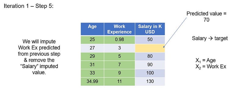
Update the predicted experience value in the missing cell in “experience” column. Now, remove “salary” imputed value. The remaining features and rows becomes the feature matrix(purple cells) and “salary” becomes the target variable(yellow cells). We will run the linear regression model on the fully filled rows with X= age and experience and Y=salary. To estimate the missing salary, we will use the missing value row (white cells) as the test data.
The predicted value for Salary is 70.
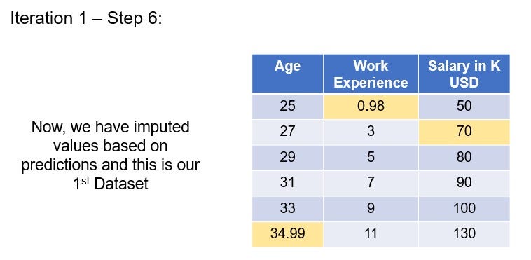
We have now imputed the missing values in the original dataset and the predicted values after 1st iteration is shown here.
Let’s name this as “First” dataset.
This is Iteration 1 which is completed.
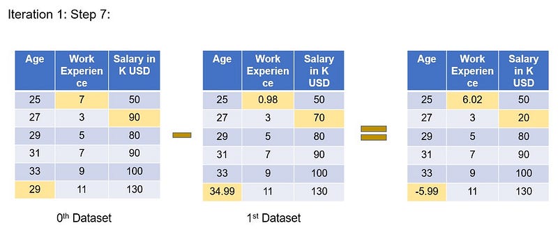
We will subtract the two datasets(zeroth and first). The resultant dataset is as shown here.
If we observe, the absolute difference between 2 datasets are higher in few imputed values. Our aim is to reduce these differences close to 0. To achieve this we have to do many iterations.
So, now we repeat the steps 2–6 with the new dataset (first), until we get a stable model. i.e. until the difference between the 2 latest imputed datasets becomes very small, close to 0.
Technically, we stop the iterations when a pre-defined threshold is breached or we can do until a pre-defined maximum number of iterations gets completed.
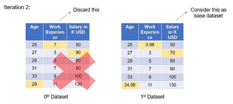
Now we will use the “first” dataset as our base dataset to do imputations, and discard the “Zeroth” dataset which had the mean imputations.
With “first” dataset as base, let’s perform all the steps 2–6 and again predict the imputed values for the initial 3 missing values.
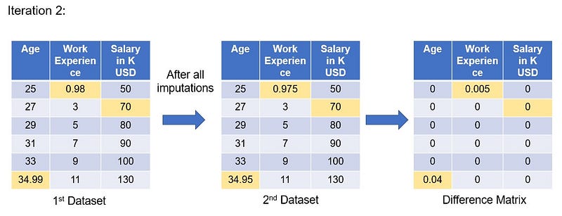
Here’s is my iteration 2 values. I took the first dataset , did all the imputations and subtracted the new dataset values form first dataset and got the difference matrix as shown.
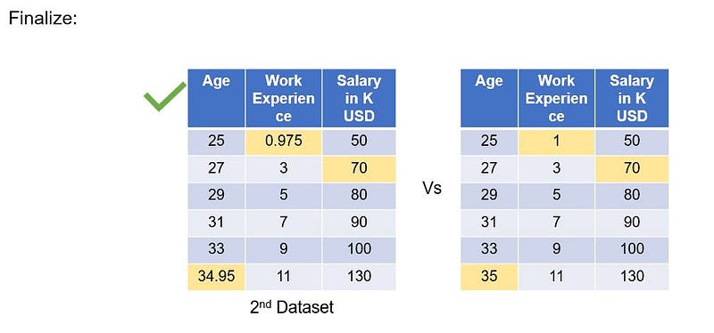
The second dataset imputed values for age is 34.95, experience is 0.975 and Salary is 70. When we compare these imputed values with the true values of the missing values which is age =35, experience = 1 and Salary = 70K, it is almost same with very small difference.
We can either stop here as we almost got the same numbers, or proceed with next iteration until we get 0 difference.
As far as this example is concerned, we will stop it here. And so, the second dataset will be the final imputed values for the missing values as shown.
Imputation by Mean/Median values:
Advantages:
- Simple and quick
- Works better with small datasets with numerical values
Disadvantages:
- Does not work well with categorical variables
- Not very accurate
- Does not account for uncertainty in the imputations
- Does not factor correlation between features. Only works well at column level.
kNN Imputation method:
Advantages:
- More accurate than mean/median imputations or most frequent imputation methods depending on the variability in the dataset.
Disadvantages:
- Computationally expensive. It works by storing entire training dataset in the memory.
- Sensitive to outliers in the dataset
To summarize, we have seen different methods to handle missing values in the dataset. Business context and domain knowledge need to be kept in mind prior to arriving at a decision strategy.
Please go through the GitHub here for code example in python.
That’s all for now. I will come back with more techniques as part of the “EDA and Feature Engineering” series. Please feel free to provide your valuable feedback or comments and clap if you like and there is some value for you.
Disclaimer: The postings here are personal point of views from my experiences, analysis, thoughts, readings from various sources.
References:


