Earnings Call Sentiment Analysis (Part I)

Predicting sentiments about future outlooks with Machine Learning in Deephaven

By Noor Malik

Every quarter, publicly-owned companies hold a conference call where they discuss their quarterly financial performance and future outlook. To investors and analysts, these calls provide valuable insight into the state of a company, which can inform their fundamental analyses and trading decisions. However, listening in on an earnings call is a time consuming process. What if the overall sentiment of an earnings call could be quickly determined in order to provide a rough idea of the company’s future outlook? In this project, I used Deephaven to explore the possibility of automating the analysis of earnings calls via a variety of Sentiment Analysis techniques.

Gathering Data

To gather training data for my sentiment analysis models, I manually scraped earnings call transcripts from the website SeekingAlpha.com. Machine learning models are typically trained on fairly large datasets, but my models would need to work with only as much data as I could manually scrape from SeekingAlpha, so I tried to find the most polarized positive and negative calls that I could in order to maximize the accuracy of my models.

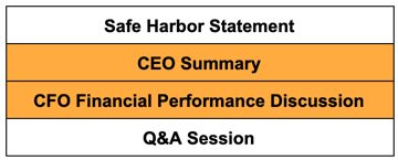
Earnings calls have four main sections: the safe-harbor statement, the CEO’s summary of the state of the company, the CFO’s discussion of the company’s quarterly financial performance, and the Q&A session. For my analysis, I used only the CEO summary and CFO financial performance discussion sections.

Ultimately, I scraped and classified 50 earnings calls: 25 positive and 25 negative. I stored the content, ticker, sentiment label, calendar year, and quarter for each call in a Deephaven user table for later use.

Text Preprocessing

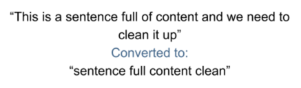
The first step in any natural language processing task is preprocessing: removing unnecessary noise and correctly formatting the text for use by your models. Below are the preprocessing measures I took on the earnings call transcripts:

• Convert all words to lowercase to avoid storing both uppercase and lowercase forms of the same word, accomplished with the lower() method in Python’s string module.
• Correct spacing problems caused by paragraph breaks (e.g., “End of sentence.Start of another” converted to “End of sentence. Start of another”). Accomplished with the sub() function in the re Python regex module.
• Remove all punctuation to avoid multiple representations of the same word, accomplished with functions in the text preprocessing Python module spacy.
• Remove stop words (common words which should be ignored, such as “a”, “an”, and “the”). Also accomplished via spacy.
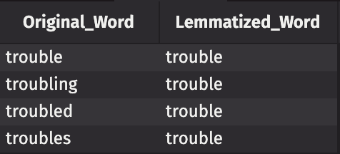
• Lemmatization (removing inflection to reduce words down to their “dictionary form”). Also accomplished via spacy.

One built-in feature of Deephaven that made preprocessing all the raw text easier was broadcasting: the process of simultaneously applying an operation to all rows of a table. Without broadcasting, I would need to loop over all rows of my table and apply the preprocessing function to each call. With broadcasting, however, cleaning all the earnings calls involved only one line of code:

cleanedCalls = rawCalls.update(“Text = (String)cleanText.call(Text)”)

Document Representations

Machine learning models work with numbers as input, not words, so the preprocessed transcripts need to be converted to numerical form. There are a variety of numerical document representations available. In this project, I used two of the most common ones: word embedding and TF-IDF.

Word Embedding

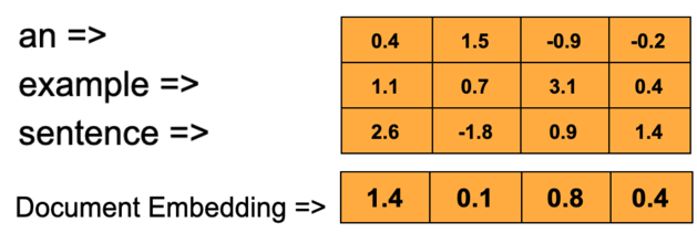
A word embedding document representation converts words into vectors of floats of a pre-specified length, called embeddings. When embeddings are used in machine learning, the float values are considered trainable parameters to be learned by the model during fitting. The model will tend to assign similar float values to words which appear together frequently, which makes embeddings capable of capturing nuanced relationships between words. Furthermore, trained embedding vectors are often “dense” (mostly containing nonzero values), which makes them effective in neural network models.

A document is represented through word embedding by first replacing each word in the document with its embedding vector, and then averaging together all the embedding vectors to obtain one vector representing the entire document:

TF-IDF

TF-IDF stands for Term Frequency — Inverse Document Frequency, which are two statistics computed for each document and multiplied together to produce the document’s “TF-IDF score” vector. Term frequency is the frequency with which a word occurs in a document: words which occur frequently in a document have high term frequency, while words which occur very few times have low term frequency. Inverse document frequency is a measure of how infrequently each word appears across all available documents: a word which appears in all documents will have an inverse document frequency of zero, while a word unique to a single document will have the maximum inverse document frequency. To compute the IDF for a given word, take the log of the total number of documents in your corpus divided by the number of documents which contain the word.

When using TF-IDF to encode documents, a vocabulary of all words in all documents is first compiled, and then for each document the TF and IDF values are computed for each word and multiplied together to produce a score vector the length of the vocabulary (note that while the TF values for each word are unique to each document, the IDF values are universal for a given set of documents):

Document A: “Earth is the third planet from the sun”

Document B: “Jupiter is the largest planet”

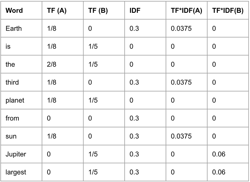
As seen in the example above, TF-IDF assigns the highest scores to the most important words in each document: “Earth”, “third”, and “sun” have high scores in document A, and “Jupiter” and “largest” have high scores in document B.

Models

After some research, I found three promising machine learning models to try: a neural network which used a pre-trained word embedding, and the Bernoulli Naive Bayes and Nearest Centroid models, which both used TF-IDF representations. I discuss my experience with each of these models below.

When testing each model, I followed a process called cross-validation, where a model is tested over many iterations with the data divided randomly into training and testing data at each iteration. Here’s how I shuffled the data on each iteration of cross-validation:

shuffled = unshuffled.update(“__r=Math.random()”).sort(“__r”).dropColumns(“__r”)

With Deephaven, I again was able to take advantage of broadcasting in the testing process. I had a function called predict(), which took two parameters, a new earnings call and a model type, and returned a prediction of 0 or 1 (negative or positive sentiment) for that new earnings call. I broadcasted the predict() function to all rows of my testing data table as follows:

testData = testData.update(“Prediction=(int)predict.call(Text, `c`)”)

Pre-Trained Embedding

Perhaps the biggest challenge I faced in this project was a lack of data: as mentioned above, while machine learning models are typically trained on thousands of training examples, I had to work with only 50 training examples. This prevented me from experimenting with complex but promising models with many learnable parameters. However, there exists a way to leverage the prediction power of highly complex models even when you have little data: transfer learning.

Transfer learning is the idea of first training a complex model for a problem very similar to yours but for which there is plenty of training data, and then simply “fine-tuning” the model to work for your specific task. For example, if your objective was to classify medical abnormalities in x-ray scans, but you had only 20 x-rays to work with, you could first train a machine learning model to classify everyday objects like animals and vehicles, for which there are millions of available images, and then retrain the few parameters corresponding to high-level features in order to fine-tune the model to your specific problem, with the assumption that low-level features which perform fundamental tasks like edge detection would be shared by both tasks.

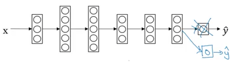
I took advantage of transfer learning by building upon a pre-trained Tensorflow document embedding model. It had 50 embedding dimensions and was trained on a corpus of billions of news articles, so I was confident that it could capture complex relationships between words. To this model, I appended a 16-node layer for fine-tuning and a single-node layer to output a prediction of whether each document had positive or negative sentiment. After testing the model over 50 iterations, reshuffling the data each time, I achieved an average classification accuracy of about 68%.

Bernoulli Naive Bayes

Naive Bayes is a machine learning model which uses the training data to estimate certain probability distributions, and then uses those distributions to compute the most likely class (in this case, positive or negative sentiment) of each training example. For this model, I used TF-IDF to represent the documents because sparse (mostly containing zeroes) TF-IDF vectors are appropriate for use in Bernoulli Naive Bayes whereas dense embedding vectors are not.

Each value in a document’s TF-IDF vector is called a “feature.” In Bernoulli Naive Bayes, a nonzero value for a specific word in a document’s TF-IDF vector would mean the document has the “feature” of that word, and a zero value would mean the document does not have the feature.

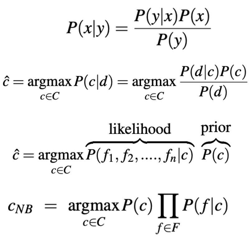
In my case, two probabilities must be compared: the probability of a new document having its specific feature vector given that the document has positive sentiment, and the same probability but given that the document has negative sentiment. The first of these probabilities is computed by finding the ratio of training examples which have positive sentiment and whose feature vectors exactly match the new document’s feature vector to the number of training examples which have positive sentiment. The second probability is simply 1 minus the first probability.

Without making any assumptions, computing these probabilities from the data is extremely difficult: if there are n features, we would need 2*(2_n — 1) unique training examples to obtain nonzero probabilities for each new document, and far more to obtain reliable estimates. This is where the “naive” part of Naive Bayes comes into play.

The “naive” assumption of Naive Bayes is shown in line four above: all the features in a TF-IDF feature vector are assumed to be conditionally independent of each other, conditioned on class. Making this independence assumption reduces the maximum number of training examples needed to only 2n. Note that this independence assumption is certainly not true in this case; positive earnings calls have groups of words like “excellent quarter” or “record sales” that are likely to appear together. However, it turns out that we can make the Naive Bayes assumption and still predict document classes with decent accuracy: testing this model over 50 iterations, reshuffling the data each time, I achieved an average classification accuracy of about 77%.

Nearest Centroid

Nearest Centroid is the simplest of the three models I tried: the idea is that given a training data set of (x, y) pairs, where x is a vector of features for a specific training example (a TF-IDF vector in this case) and y is the label for that specific training example (positive or negative sentiment in this case), compute the mean of the x vectors for each label y, and classify each new example to have the same label as its closest mean vector, or centroid.

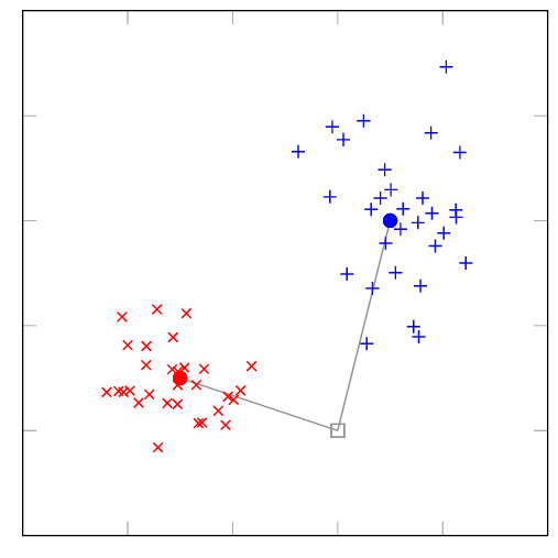
Because the red centroid is closer to the square, the predicted label for the square is red.

Testing this model over 50 iterations, reshuffling the data each time, I achieved an average classification accuracy of about 82%.

Conclusion

To my surprise, the simplest of the three models I tried ended up being the best predictor of the sentiments of earnings calls. Research shows that humans tend to agree on the sentiment of a given text about 70–85% of the time, so a model with 82% accuracy is respectable. As mentioned several times, the biggest bottleneck in this project was a lack of data: I believe that with sufficient data, the Transfer Learning based model, having a significant number of trainable parameters, will perform best.

In Part 2 of this project, I plan to use my centroid model to make predictions on live data retrieved from an RSS feed of new earnings call transcripts.

References

[1] Deeplearning.ai. “Transfer Learning (C3W2L07),” YouTube, Aug. 25, 2017 [Video file]. Available: https://www.youtube.com/watch?v=yofjFQddwHE. [Accessed: Jun. 26, 2020].

[2] D. Jurafsky and J. Martin, Speech and Language Processing, 3rd ed., 2019, pp. 58–59.

[3] Adcock, Jeremy & Allen, Euan & Day, Matthew & Frick, Stefan & Hinchliff, Janna & Johnson, Mack & Morley-Short, Sam & Pallister, Sam & Price, Alasdair & Stanisic, Stasja. (2015). Advances in quantum machine learning.