Dyna-Q: Bridging Simulation and Experience in Reinforcement Learning (Pac-Man)

Introduction

In the diverse landscape of reinforcement learning (RL), the Dyna-Q algorithm stands out as a pioneering approach that synergistically combines direct experience with simulated learning. Developed by Richard S. Sutton, Dyna-Q addresses one of the fundamental challenges in RL: efficiently utilizing limited interactions with the environment to accelerate learning and improve decision-making. This essay delves into the principles of Dyna-Q, its operational framework, applications, and the broader implications for the field of reinforcement learning.

In the labyrinth of learning, every step taken illuminates a new path, blending experience with imagination to navigate the unknown.

Foundations of Dyna-Q

Dyna-Q is predicated on the insight that learning from actual experience, while crucial, is inherently limited by the opportunities for interaction with the environment. This limitation becomes particularly pronounced in complex or hazardous environments where exhaustive exploration is impractical or impossible. Dyna-Q circumvents this constraint by supplementing real-world experience with numerous simulated experiences, thereby amplifying the learning opportunities.

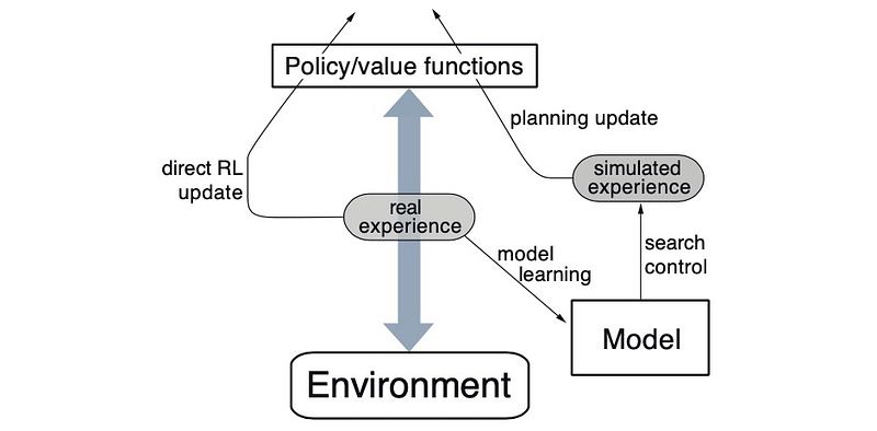
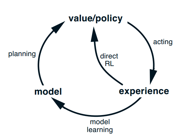
The core components of Dyna-Q include:

• Direct Learning from Real Experience: Similar to traditional RL algorithms, Dyna-Q learns from real interactions with the environment, updating its policy based on the outcomes of its actions.
• Model Learning: Concurrently, Dyna-Q constructs a model of the environment based on observed transitions, capturing the dynamics of how the environment responds to actions.
• Simulation-Based Learning: Leveraging the learned model, Dyna-Q conducts simulations of interactions with the environment, enabling the agent to learn from hypothetical scenarios alongside actual experiences.

Operational Framework

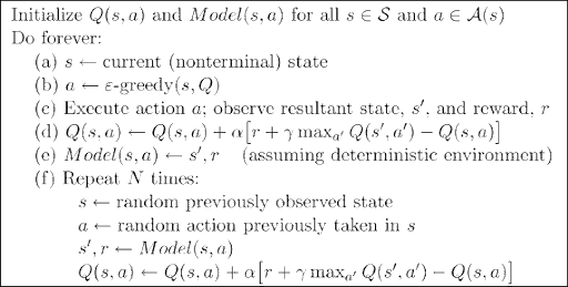
The operational cycle of Dyna-Q can be summarized in several key steps:

1. Execute and Learn: The agent takes an action in the real environment, observes the outcome, and updates its policy based on the actual experience.
2. Model Building: From the observed state transition and reward, the agent updates its internal model of the environment, refining its understanding of the environmental dynamics.
3. Simulation: The agent uses its model to simulate numerous additional experiences, generating synthetic state transitions and rewards for various actions.
4. Policy Update: The agent updates its policy based on both real and simulated experiences, effectively learning as if it had interacted with the environment more extensively.

This iterative process enables Dyna-Q to exploit the acquired knowledge to the fullest extent, significantly accelerating the learning process.

Applications and Implications

Dyna-Q’s ability to enhance learning efficiency through simulation has found applications across a range of domains, from robotics, where it enables safer and faster development of control policies, to game playing, where exhaustive exploration of the game space is computationally prohibitive. Furthermore, Dyna-Q’s model-based approach facilitates planning and decision-making under uncertainty, making it valuable for logistics, operations research, and financial modeling.

The conceptual innovation of Dyna-Q has also spurred further research into model-based reinforcement learning, leading to the development of more sophisticated algorithms that balance the trade-offs between model accuracy, computational efficiency, and the benefits of simulation.

Challenges and Future Directions

Despite its advantages, Dyna-Q faces challenges related to model accuracy and computational demands. The effectiveness of simulated learning hinges on the fidelity of the model, with inaccuracies potentially leading to suboptimal policies. Moreover, the computational cost of maintaining and querying the model, along with executing numerous simulations, can become prohibitive as the complexity of the environment increases.

Addressing these challenges, ongoing research explores adaptive modeling techniques, efficient simulation strategies, and hybrid approaches that dynamically balance direct and simulated learning. Additionally, the integration of deep learning with Dyna-Q offers promising avenues for scaling model-based reinforcement learning to more complex environments.

Code

Implementing a complete Dyna-Q algorithm for a Pac-Man game involves several steps, including setting up the environment, defining the learning algorithm, and evaluating performance. While it’s complex to build and run a full Pac-Man game here, I’ll provide a simplified example that captures the essence of Dyna-Q. This example will be based on a grid world that represents a very basic version of a Pac-Man-like environment, focusing on the key components of the Dyna-Q algorithm: direct learning from interaction, model learning, and planning/simulation based on the learned model.

Environment Setup

This simplified grid world consists of a Pac-Man starting position, a goal position (representing the point to reach), and obstacles. Pac-Man can move up, down, left, or right, attempting to reach the goal while avoiding obstacles.

Dyna-Q Algorithm

The Dyna-Q algorithm involves:

1. Learning from real actions in the environment (Direct Learning).
2. Building a model of the environment’s dynamics (Model Learning).
3. Planning by simulating actions in the built model (Planning/Simulation).

import numpy as np

# Environment settings
grid_size = (5, 5)
start_position = (0, 0)
goal_position = (4, 4)
obstacle_positions = [(1, 1), (2, 2), (3, 3)]
actions = [(-1, 0), (1, 0), (0, -1), (0, 1)]  # Up, Down, Left, Right
n_actions = len(actions)

# Helper functions
def to_state(position):
    return position[0] * grid_size[1] + position[1]

def from_state(state):
    return (state // grid_size[1], state % grid_size[1])

def step(position, action):
    next_position = (position[0] + action[0], position[1] + action[1])
    if next_position[0] < 0 or next_position[0] >= grid_size[0] or next_position[1] < 0 or next_position[1] >= grid_size[1] or next_position in obstacle_positions:
        return position, -1  # Hit boundary or obstacle
    elif next_position == goal_position:
        return next_position, 10  # Reached goal
    return next_position, 0  # Normal move

# Initialize Q-table and model
Q = np.zeros((grid_size[0] * grid_size[1], n_actions))
model = {}  # For storing transitions (s, a) -> (s', r)

# Dyna-Q parameters
alpha = 0.1
gamma = 0.95
epsilon = 0.1
n_planning_steps = 5

# Learning and planning loop
for episode in range(1000):
    state = to_state(start_position)
    while state != to_state(goal_position):
        # Epsilon-greedy action selection
        if np.random.rand() < epsilon:
            action_index = np.random.choice(n_actions)
        else:
            action_index = np.argmax(Q[state])
        
        # Take action and observe the outcome
        next_position, reward = step(from_state(state), actions[action_index])
        next_state = to_state(next_position)
        
        # Direct learning
        Q[state, action_index] += alpha * (reward + gamma * np.max(Q[next_state]) - Q[state, action_index])
        
        # Model learning
        model[(state, action_index)] = (next_state, reward)
        
        # Planning with simulated experiences
        for _ in range(n_planning_steps):
            simulated_state, simulated_action = list(model.keys())[np.random.choice(len(model))]
            simulated_next_state, simulated_reward = model[(simulated_state, simulated_action)]
            Q[simulated_state, simulated_action] += alpha * (simulated_reward + gamma * np.max(Q[simulated_next_state]) - Q[simulated_state, simulated_action])
        
        state = next_state

# Simple function to visualize the policy
def visualize_policy(Q):
    directions = ['↑', '↓', '←', '→']
    policy = np.array([directions[np.argmax(Q[to_state((i, j))])] for i in range(grid_size[0]) for j in range(grid_size[1])]).reshape(grid_size)
    print(policy)

visualize_policy(Q)

This script initializes the environment, defines the Dyna-Q learning and planning process, and iteratively updates the Q-values based on both real interactions and simulated experiences from the learned model. The visualize_policy function provides a simple textual representation of the learned policy, showing the best action to take in each grid cell.

[['↓' '←' '←' '←' '←']
 ['↓' '↑' '↑' '↑' '↑']
 ['↓' '↓' '↑' '↑' '↑']
 ['→' '→' '↓' '↑' '↑']
 ['↑' '↑' '→' '→' '↑']]

Creating a plot to visualize Pac-Man’s movement through the grid using the Dyna-Q algorithm involves tracking Pac-Man’s path as it follows the policy learned during training. This example extends the previous Dyna-Q implementation to include visualization of the movement. We’ll use Matplotlib to create a static plot showing the path from the starting position to the goal. We’ll modify the end of the Dyna-Q script to track Pac-Man’s path during an episode and then plot this path:

import matplotlib.pyplot as plt

# Function to visualize the grid and path
def plot_grid_and_path(start, goal, obstacles, path):
    fig, ax = plt.subplots()
    
    # Create grid
    ax.set_xlim(0, grid_size[1])
    ax.set_ylim(0, grid_size[0])
    plt.grid(which='both')
    
    # Plot start, goal, and obstacles
    ax.plot(start[1]+0.5, start[0]+0.5, 'go')  # Start in green
    ax.plot(goal[1]+0.5, goal[0]+0.5, 'ro')  # Goal in red
    for obs in obstacles:
        ax.plot(obs[1]+0.5, obs[0]+0.5, 'ks')  # Obstacles in black squares
    
    # Plot path
    for pos in path:
        ax.plot(pos[1]+0.5, pos[0]+0.5, 'bo')  # Path in blue dots
    
    plt.show()

# Run an episode to get the path using the learned Q-values
def get_path(Q, start_position, goal_position):
    state = to_state(start_position)
    path = [from_state(state)]
    while state != to_state(goal_position):
        action_index = np.argmax(Q[state])
        next_position, _ = step(from_state(state), actions[action_index])
        path.append(next_position)
        state = to_state(next_position)
        if len(path) > grid_size[0]*grid_size[1]:  # Prevent infinite loops
            break
    return path

path = get_path(Q, start_position, goal_position)

# Plot the movement
plot_grid_and_path(start_position, goal_position, obstacle_positions, path)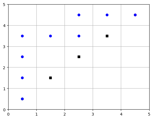

Creating an animation to visualize Pac-Man’s movement through the grid using the learned Dyna-Q policy is possible. We can use the matplotlib.animation module to create an animation where Pac-Man moves from the starting point to the goal, based on the path determined by the learned policy. Below is a step-by-step guide to create such an animation. This builds upon the previous code examples, assuming you already have the grid setup, obstacles, and a learned Q-table from running the Dyna-Q algorithm. We’ll modify the previous code to include animation functionality. This example assumes you’ve already obtained the optimal path using the learned Q-values as shown in the previous steps.

import matplotlib.pyplot as plt
from matplotlib.animation import FuncAnimation

# Initialize the plot for animation
fig, ax = plt.subplots()
ax.set_xlim(0, grid_size[1])
ax.set_ylim(0, grid_size[0])
plt.xticks(range(grid_size[1]))
plt.yticks(range(grid_size[0]))
ax.grid(True)
plt.gca().invert_yaxis()  # Invert y-axis to match grid representation

# Plot obstacles and goal
for obs in obstacle_positions:
    ax.add_patch(plt.Rectangle((obs[1], obs[0]), 1, 1, color='black'))
ax.add_patch(plt.Rectangle((goal_position[1], goal_position[0]), 1, 1, color='red'))

# Initialize Pac-Man's position as a yellow circle
pacman, = ax.plot([], [], 'yo', markersize=12)

# Extract the path from the Q-table (assumed to be obtained already)
path = get_path(Q, start_position, goal_position)  # Re-use get_path function from previous step

# Animation update function
def update(frame):
    pos = path[frame]
    pacman.set_data(pos[1] + 0.5, pos[0] + 0.5)
    return (pacman,)

# Create the animation
ani = FuncAnimation(fig, update, frames=len(path), blit=True, interval=200)

plt.show()

The code above will display the animation in a Jupyter notebook or a Python script run in an environment that supports graphical output. If you want to save the animation to a file, you can do so by adding the following line after creating the ani object, ensuring you have the necessary writer installed (e.g., ffmpeg or imagemagick):

ani.save('pacman_movement.mp4', writer='ffmpeg', fps=2)

or for GIF format:

ani.save('pacman_movement.gif', writer='imagemagick', fps=2)

Notes

This example is highly simplified and doesn’t include features of a full Pac-Man game, like ghosts or multiple goals (dots). Dyna-Q’s strength in planning and learning from simulated experiences can be applied to more complex environments, provided a suitable model of the environment’s dynamics can be learned or approximated.

• This animation represents Pac-Man navigating through the grid based on the learned policy, moving from the start position to the goal while avoiding obstacles.
• The path used in the animation should be pre-computed using the Dyna-Q algorithm to reflect the policy’s performance accurately.
• The animation setup provided here is basic and intended for demonstration purposes. You might need to adjust the code based on your specific environment setup, library versions, and Python environment capabilities.

Conclusion

Dyna-Q represents a seminal advancement in reinforcement learning, embodying the principle that learning can be dramatically enhanced by intelligently blending experience with imagination. By harnessing the power of simulation, Dyna-Q accelerates the acquisition of knowledge and the refinement of policies, showcasing the potential of model-based approaches in overcoming the limitations of direct experience. As reinforcement learning continues to evolve, the legacy of Dyna-Q endures, guiding the exploration of innovative strategies that combine the richness of real-world interaction with the boundless possibilities of simulated experience.